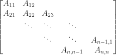
A tridiagonal matrix is a square matrix whose elements are zero away from the main diagonal, the subdiagonal, and the superdiagonal. In other words, it is a banded matrix with upper and lower bandwidths both equal to 

An important example is the matrix 

![\notag T_5 = \left[ \begin{array}{@{}*{4}{r@{\mskip10mu}}r} 4 & -1 & & & \\ -1 & 4 & -1 & & \\ & -1 & 4 & -1 & \\ & & -1 & 4 & -1 \\ & & & -1 & 4 \end{array}\right].](https://s0.wp.com/latex.php?latex=%5Cnotag++++T_5+%3D+%5Cleft%5B++++%5Cbegin%7Barray%7D%7B%40%7B%7D%2A%7B4%7D%7Br%40%7B%5Cmskip10mu%7D%7Dr%7D+++++++++++++++++4++%26+-1+%26++++%26++++%26++++%5C%5C+++++++++++++++++-1+%26+4++%26+-1+%26++++%26++++%5C%5C++++++++++++++++++++%26+-1+%26+4++%26+-1+%26++++%5C%5C++++++++++++++++++++%26++++%26+-1+%26+4++%26+-1+%5C%5C++++++++++++++++++++%26++++%26++++%26+-1+%26+4++++%5Cend%7Barray%7D%5Cright%5D.+&bg=ffffff&fg=222222&s=0&c=20201002)
It is symmetric positive definite, diagonally dominant, a Toeplitz matrix, and an 
Tridiagonal matrices have many special properties and various algorithms exist that exploit their structure.
Symmetrization
It can be useful to symmetrize a matrix by transforming it with a diagonal matrix. The next result shows when symmetrization is possible by similarity.
Theorem 1. If
is tridiagonal and
for all
then there exists a diagonal
with positive diagonal elements such that
is symmetric, with
element
.
Proof. Let
. Equating
and
or
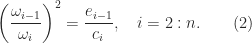
As long as
and solve (2) to obtain real, positive
,
. The formula for the off-diagonal elements of the symmetrized matrix follows from (1) and (2).

LU Factorization
The LU factors of a tridiagonal matrix are bidiagonal:

The equation 

The recurrence breaks down with division by zero if one of the leading principal submatrices 


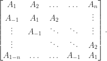
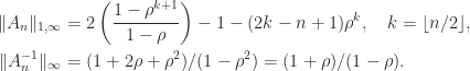
For a tridiagonal Toeplitz matrix
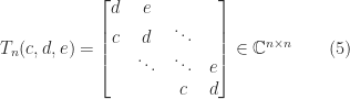
the elements of the LU factors converge as 

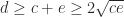
Theorem 2. Suppose that
has an LU factorization with LU factors (3) and that
and
. Then
decreases monotonically and
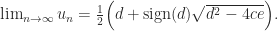
From (4), it follows that under the conditions of Theorem 2, 


Inverse
The inverse of a tridiagonal matrix is full, in general. For example,
![\notag T_5(-1,3,-1)^{-1} = \left[\begin{array}{rrrrr} 3 & -1 & 0 & 0 & 0\\ -1 & 3 & -1 & 0 & 0\\ 0 & -1 & 3 & -1 & 0\\ 0 & 0 & -1 & 3 & -1\\ 0 & 0 & 0 & -1 & 3 \end{array}\right]^{-1} = \frac{1}{144} \left[\begin{array}{ccccc} 55 & 21 & 8 & 3 & 1 \\ 21 & 63 & 24 & 9 & 3 \\ 8 & 24 & 64 & 24 & 8 \\ 3 & 9 & 24 & 63 & 21\\ 1 & 3 & 8 & 21 & 55 \end{array}\right].](https://s0.wp.com/latex.php?latex=%5Cnotag+++T_5%28-1%2C3%2C-1%29%5E%7B-1%7D+++%3D+%5Cleft%5B%5Cbegin%7Barray%7D%7Brrrrr%7D+3+%26+-1+%26+0+%26+0+%26+0%5C%5C+++++++++++++++++++++++++++++++-1+%26+3+%26+-1+%26+0+%26+0%5C%5C+++++++++++++++++++++++++++++++0+%26+-1+%26+3+%26+-1+%26+0%5C%5C+++++++++++++++++++++++++++++++0+%26+0+%26+-1+%26+3+%26+-1%5C%5C+++++++++++++++++++++++++++++++0+%26+0+%26+0+%26+-1+%26+3+%5Cend%7Barray%7D%5Cright%5D%5E%7B-1%7D++%3D++%5Cfrac%7B1%7D%7B144%7D+++++%5Cleft%5B%5Cbegin%7Barray%7D%7Bccccc%7D+55+%26+21+%26+8++%26+3++%26+1+%5C%5C++++++++++++++++++++++++++++++++21+%26+63+%26+24+%26+9++%26+3+%5C%5C++++++++++++++++++++++++++++++++8+%26+24+%26+64+%26+24+%26+8+%5C%5C+3+%26+9+%26+24+%26+63+%26+21%5C%5C++++++++++++++++++++++++++++++++1+%26+3++%26+8++%26+21+%26+55+%5Cend%7Barray%7D%5Cright%5D.+&bg=ffffff&fg=222222&s=0&c=20201002)
Since an 


Theorem 3. If
is tridiagonal, nonsingular, and irreducible then there are vectors
,
,
, and
, all of whose elements are nonzero, such that
![\notag (A^{-1})_{ij} = \begin{cases} u_iv_j, & i\le j,\\ x_iy_j, & i\ge j.\\[4pt] \end{cases}](https://s0.wp.com/latex.php?latex=%5Cnotag+++++++++++%28A%5E%7B-1%7D%29_%7Bij%7D+%3D+%5Cbegin%7Bcases%7D+++++++++++++++++++++++++++++++++u_iv_j%2C+%26+i%5Cle+j%2C%5C%5C+++++++++++++++++++++++++++++++++x_iy_j%2C+%26+i%5Cge+j.%5C%5C%5B4pt%5D+++++++++++++++++++++++++++%5Cend%7Bcases%7D+&bg=ffffff&fg=222222&s=0&c=20201002)
The theorem says that the upper triangle of the inverse agrees with the upper triangle of a rank-

If a tridiagonal matrix 

where 

in which the 

The inverse of the Toeplitz tridiagonal matrix 
Eigenvalues
The most widely used methods for finding eigenvalues and eigenvectors of Hermitian matrices reduce the matrix to tridiagonal form by a finite sequence of unitary similarity transformations and then solve the tridiagonal eigenvalue problem. Tridiagonal eigenvalue problems also arise directly, for example in connection with orthogonal polynomials and special functions.
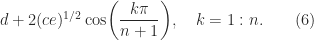
The eigenvalues of the Toeplitz tridiagonal matrix
The eigenvalues are also known for certain variations of the symmetric matrix 


Some special results hold for the eigenvalues of general tridiagonal matrices. A matrix is derogatory if an eigenvalue appears in more than one Jordan block in the Jordan canonical form, and nonderogatory otherwise.
Theorem 4. If
Proof. Let
, for any
. The matrix
is lower triangular with nonzero diagonal elements
and hence it is nonsingular. Therefore
has rank at least
for all
when
Corollary 5. If
Proof. By Theorem 1 the eigenvalues of
and so are real. The matrix
is tridiagonal and irreducible so it is nonderogatory by Theorem 4, which means that its eigenvalues are simple because it is symmetric.
The formula (6) confirms the conclusion of Corollary 5 for tridiagonal Toeplitz matrices.
Corollary 5 guarantees that the eigenvalues are distinct but not that they are well separated. The spacing of the eigenvalues in (6) clearly reduces as 

For example,
![\notag W_5^+ = \left[\begin{array}{ccccc} 2 & 1 & 0 & 0 & 0\\ 1 & 1 & 1 & 0 & 0\\ 0 & 1 & 0 & 1 & 0\\ 0 & 0 & 1 & 1 & 1\\ 0 & 0 & 0 & 1 & 2 \end{array}\right].](https://s0.wp.com/latex.php?latex=%5Cnotag+++W_5%5E%2B+%3D+%5Cleft%5B%5Cbegin%7Barray%7D%7Bccccc%7D+2+%26+1+%26+0+%26+0+%26+0%5C%5C+1+%26+1+%26+1+%26+0+%26+0%5C%5C+0+%26+1+%26+0+%26+1+%26+0%5C%5C+0+%26+0+%26+1+%26+1+%26+1%5C%5C+0+%26+0+%26+0+%26+1+%26+2+%5Cend%7Barray%7D%5Cright%5D.+&bg=ffffff&fg=222222&s=0&c=20201002)
Here are the two largest eigenvalues of 
>> A = anymatrix('matlab/wilkinson',21);
>> e = eig(A); e([20 21])
ans =
  10.746194182903322
  10.746194182903393
These eigenvalues (which are correct to the digits shown) agree almost to the machine precision.
Notes
Theorem 2 is obtained for symmetric matrices by Malcolm and Palmer (1974), who suggest saving work in computing the LU factorization by setting 


A sample reference for Theorem 3 is Ikebe (1979), which is one of many papers on inverses of banded matrices.
The eigenvectors of a symmetric tridiagonal matrix satisfy some intricate relations; see Parlett (1998, sec. 7.9).
References
This is a minimal set of references, which contain further useful references within.
- Murray Dow, Explicit Inverses of Toeplitz and Associated Matrices, ANZIAM J. 44, E185–E215, 2003.
- Robert Gregory and David Karney, A Collection of Matrices for Testing Computational Algorithms, Wiley, 1969.
- Yasuhiko Ikebe, On inverses of Hessenberg matrices. Linear Algebra Appl., 24:93–97, 1979.
- Michael A. Malcolm and John Palmer, A Fast Method for Solving a Class of Tridiagonal Linear Systems, Comm. ACM 17, 14–17, 1974.
- Beresford Parlett, The Symmetric Eigenvalue Problem, Society for Industrial and Applied Mathematics, Philadelphia, PA, USA, 1998.
- J. H. Wilkinson, The Algebraic Eigenvalue Problem, Oxford University Press, 1965, Section 5.45.
 of vectors
  . The unblocked algorithm


 , as
, as
 % Compute by the unblocked algorithm.
 of
of  . The natural computation is, from the definition of matrix multiplication, the “point algorithm”


 ,
,  , and
, and  be partitioned into blocks of size
  is assumed to be an integer. The blocked computation is


 flops on about
  data, whereas the point algorithm performs
  flops on
  flops on
  flops-to-data ratio that gives the blocked algorithm its advantage, because it masks the memory access costs.
 ,
,  , and
, and  become
  ,
,  , and
, and  ). It usually computes a block factorization, in which a matrix property based on the nonzero structure becomes the corresponding property blockwise; in particular, the scalars 0 and 1 become the zero matrix and the identity matrix, respectively.
 matrix
 ![\notag A = \left[ \begin{tabular}{cc|cc} 1 & & & \\ x & 1 & & \\ \hline x & x & 1 & \\ x & x & x & 1 \end{tabular} \right] \left[ \begin{tabular}{cc|cc} x & x & x & x \\ & x & x & x \\ \hline & & x & x \\ & & & x \end{tabular} \right].](https://s0.wp.com/latex.php?latex=%5Cnotag++++A+%3D++%5Cleft%5B+%5Cbegin%7Btabular%7D%7Bcc%7Ccc%7D++++++++++++++++++1+%26+++%26++++%26++++%5C%5C++++++++++++++++++x+%26+1+%26++++%26++++%5C%5C++%5Chline++++++++++++++++++x+%26+x+%26++1+%26++++%5C%5C++++++++++++++++++x+%26+x+%26++x+%26+1+++++++++++++++++%5Cend%7Btabular%7D++%5Cright%5D++++++%5Cleft%5B+%5Cbegin%7Btabular%7D%7Bcc%7Ccc%7D++++++++++++++++++x+%26+x+%26++x+%26+x++%5C%5C++++++++++++++++++++%26+x+%26++x+%26+x++%5C%5C++%5Chline++++++++++++++++++++%26+++%26++x+%26+x++%5C%5C++++++++++++++++++++%26+++%26++++%26+x+++++++++++++++++%5Cend%7Btabular%7D++%5Cright%5D.+&bg=ffffff&fg=222222&s=0&c=20201002)
![\notag A = \left[ \begin{tabular}{cc|cc} 1 & 0 & & \\ 0 & 1 & & \\ \hline x & x & 1 & 0 \\ x & x & 0 & 1 \end{tabular} \right] \left[ \begin{tabular}{cc|cc} x & x & x & x \\ x & x & x & x \\ \hline & & x & x \\ & & x & x \end{tabular} \right].](https://s0.wp.com/latex.php?latex=%5Cnotag++++A+++%3D++%5Cleft%5B+%5Cbegin%7Btabular%7D%7Bcc%7Ccc%7D++++++++++++++++++1+%26+0+%26++++%26++++%5C%5C++++++++++++++++++0+%26+1+%26++++%26++++%5C%5C++%5Chline++++++++++++++++++x+%26+x+%26++1+%26+0++%5C%5C++++++++++++++++++x+%26+x+%26++0+%26+1+++++++++++++++++%5Cend%7Btabular%7D++%5Cright%5D++++++%5Cleft%5B+%5Cbegin%7Btabular%7D%7Bcc%7Ccc%7D++++++++++++++++++x+%26+x+%26++x+%26+x++%5C%5C++++++++++++++++++x+%26+x+%26++x+%26+x++%5C%5C++%5Chline++++++++++++++++++++%26+++%26++x+%26+x++%5C%5C++++++++++++++++++++%26+++%26++x+%26+x+++++++++++++++++%5Cend%7Btabular%7D++%5Cright%5D.+&bg=ffffff&fg=222222&s=0&c=20201002)
 satisfying
 with equality if and only if
  (nonnegativity),
 for all
  ,
,  (homogeneity),
 for all
  (the triangle inequality).
 the corresponding subordinate matrix norm on
  is defined by
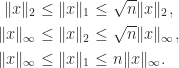
 -vector norms it can be shown that
 denotes the largest singular value of
  -norm no explicit formula is known for
  for
for  .
.

 , whereas
  for any subordinate norm), but it is consistent.
 for any unitary matrices
  . For the Frobenius norm the invariance follows easily from the trace formula.
 such that
  for
for 
 is the spectral radius (the largest absolute value of any eigenvalue). To prove this inequality, let
 ![X=[x,x,\dots,x] \in \mathbb{C}^{n\times n}](https://s0.wp.com/latex.php?latex=X%3D%5Bx%2Cx%2C%5Cdots%2Cx%5D+%5Cin+%5Cmathbb%7BC%7D%5E%7Bn%5Ctimes+n%7D&bg=ffffff&fg=222222&s=0&c=20201002) . Then
. Then  , so
, so  , giving
  since
since  . For a subordinate norm it suffices to take norms in the equation
  .
.
 , where the first two equalities are obtained from the singular value decomposition and we have used (1).
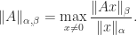
 .
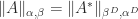
. is given in the next result. Recall that
  denotes the dual of the vector norm
  .
.
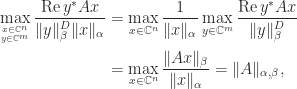
 . Here,
  denotes
  .
. .
.
 – and
– and  -norms to be the same
  , where
  (giving, in particular,
  and
and  , which are easily obtained directly).
 norm when
 ,
,


 , where the maximum is attained for
  . For (4), using the Hölder inequality,
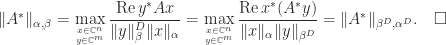
 th row of
  .
. . The unit cube
  , where
 ![e = [1,1,\dots,1]^T](https://s0.wp.com/latex.php?latex=e+%3D+%5B1%2C1%2C%5Cdots%2C1%5D%5ET&bg=ffffff&fg=222222&s=0&c=20201002) , is a convex polyhedron, so any point within it is a convex combination of the vertices, which are the elements of
, is a convex polyhedron, so any point within it is a convex combination of the vertices, which are the elements of  . Hence
  implies
 , but trivially
  and (5) follows.
 . Then, using a Cholesky factorization
  (which exists even if
 we have
 . Hence
  , using (5).

 -norm has recently found use in statistics (Cape, Tang, and Priebe, 2019), the motivation being that because it satisfies
 and so can be a better norm to use in bounds. The
  -norms are used by Rebrova and Vershynin (2018) in bounding the
  and
and  ) norm is not consistent, but for any vector norm
  , we have
 . This class of matrices includes magic squares and doubly stochastic matrices. We have
  , so
, so  by (2). But
  for the vector
  of
of  by (1). Hence
  . In fact,
  for all
 ![p\in[1,\infty]](https://s0.wp.com/latex.php?latex=p%5Cin%5B1%2C%5Cinfty%5D&bg=ffffff&fg=222222&s=0&c=20201002) (see Higham (2002, Prob. 6.4) and Stoer and Witzgall (1962)).
(see Higham (2002, Prob. 6.4) and Stoer and Witzgall (1962)). ,
,  , or
, or  , for example, and we may wish to compute the norm without forming
  15.2). The power method accesses
  -norm and the
  -norm, which we compare with the
 ![p \in[1,25]](https://s0.wp.com/latex.php?latex=p+%5Cin%5B1%2C25%5D&bg=ffffff&fg=222222&s=0&c=20201002) . This shape of curve is typical, because, as the plot in the lower half indicates,
. This shape of curve is typical, because, as the plot in the lower half indicates,  is a convex function of
  for
for  (see Higham, 2002, Sec.
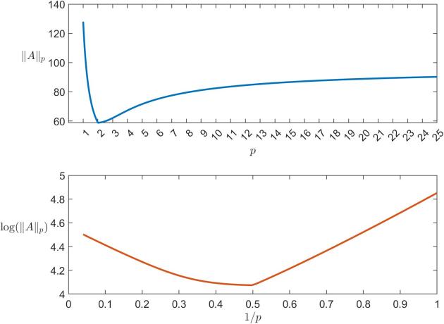
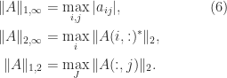
 norm, which is the max norm in (6), is investigated by Higham and Relton (2016) and extended to estimate the
  or
or  .
. can be defined by

 for all
  independent of
 ![[1.33,1.41]](https://s0.wp.com/latex.php?latex=%5B1.33%2C1.41%5D&bg=ffffff&fg=222222&s=0&c=20201002) , or
, or ![[1.67,1.79]](https://s0.wp.com/latex.php?latex=%5B1.67%2C1.79%5D&bg=ffffff&fg=222222&s=0&c=20201002) for the analogous inequality for real data. See Friedland, Lim, and Zhang (2018) and the references therein.
for the analogous inequality for real data. See Friedland, Lim, and Zhang (2018) and the references therein. is due to Rohn (2000), who shows that evaluating it is NP-hard. For general
 satisfying
 with equality if and only if
  (nonnegativity),
 for all
  (homogeneity),
 for all
  (the triangle inequality).
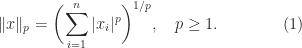
 and is given by


 , in which we are maximizing a continuous function over a compact set. Importantly, the dual of the dual norm is the original norm (Horn and Johnson, 2013, Thm.

 -norm, where

 is used to denote the number of nonzero entries in
  . In portfolio optimization, if
  specifies how much to invest in stock
  says “invest in at most
  and
and  there exist positive constants
  and
and  such that
 , then
  .
. . One can simply use the formula
  , but this requires two passes over the data (the first to evaluate
  ). For more efficient one-pass algorithms for the
  .
. .
. are totally nonnegative then so is
 ![\alpha = [\alpha_1,\alpha_2,\dots,\alpha_k]](https://s0.wp.com/latex.php?latex=%5Calpha+%3D+%5B%5Calpha_1%2C%5Calpha_2%2C%5Cdots%2C%5Calpha_k%5D&bg=ffffff&fg=222222&s=0&c=20201002) is an index vector of order
is an index vector of order  satisfying
  . If
. If  , respectively, then
  denotes the
  matrix with (
 ) element
  .
. , and
, and  then
then
 , (1) reduces to the well-known relation
  , while when
  , (1) reduces to the definition of matrix multiplication.
 comprises the indices not in
 , with
  . The Hilbert matrix is a particular case of a Cauchy matrix
  , with
  for given vectors
  . A Cauchy matrix is totally positive if
  and
and  , which follows from the formula

 satisfy
 is defined by
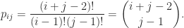
 with off-diagonal elements given by
  with
with  , illustrated by
![A([1,2],[2,3]) = \bigl[\begin{smallmatrix} \theta & \theta \\ 1 & \theta \end{smallmatrix}\bigr]](https://s0.wp.com/latex.php?latex=A%28%5B1%2C2%5D%2C%5B2%2C3%5D%29+%3D++++%5Cbigl%5B%5Cbegin%7Bsmallmatrix%7D++++%5Ctheta+%26+%5Ctheta+%5C%5C++++1++++++%26+%5Ctheta++++%5Cend%7Bsmallmatrix%7D%5Cbigr%5D+&bg=ffffff&fg=222222&s=0&c=20201002) has nonpositive determinant. However, the
has nonpositive determinant. However, the  , with
 with all elements
  by
by
 zero eigenvalues, which appear in a single Jordan block, and its largest eigenvalue is
  . In MATLAB, this matrix can be generated by
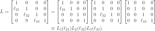
 ,
,  , and
, and  are totally nonnegative, so
  , we have
 , where
 denotes the submatrix of
  has a checkerboard (alternating) sign pattern. Indeed, we can write
  , where
  and
and  such that
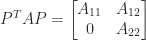
 and
and  are square, nonempty submatrices.
 . It is known that the eigenvector
  has
has  sign changes, that is,
  and (
and ( have opposite signs for
  , we already know from Perron–Frobenius theory that there is a positive eigenvector
  . This result is illustrated by the Pascal matrix above:
 is totally positive for some positive integer
 .
. for
for  , which guarantees the existence of an LU factorization. That the elements of
  and computes
  , since
  . Thus
  ,
,  . For
. For  ,
,  ; for
; for  ,
,  . Thus
  for all
  and hence
  . But
. But  , so
, so  .
. and
and  will have nonnegative elements and so from the standard backward error result for LU factorization,

 and hence

 is a diagonal matrix with positive diagonal entries and
  and
and  are unit lower and unit upper bidiagonal matrices, respectively, with the first
  entries along the subdiagonal of
  zero and the rest nonnegative.
 subdiagonal entries of
  principal minors (ones based on submatrices centred on the diagonal) and
  minors in total. However, it is not necessary to check all these minors to test for total positivity.
 for all index vectors
 ![[1,2,\dots,k]](https://s0.wp.com/latex.php?latex=%5B1%2C2%2C%5Cdots%2Ck%5D&bg=ffffff&fg=222222&s=0&c=20201002) and the entries of the other are
and the entries of the other are  minors need to be tested. Gasca and Peña have also show that total nonnegativity can be tested by checking about
  minors. A more efficient way to test for total nonnegativity is to compute the factorization in Theorem 6 and check the signs of the entries.
 the spectral radius of
  .
. ,
, ,
, for any eigenvalue
  .
. , is called the Perron vector.
![A = \bigl[\begin{smallmatrix}0 & 1 \\ 0 & 0 \end{smallmatrix}\bigr]](https://s0.wp.com/latex.php?latex=A+%3D+%5Cbigl%5B%5Cbegin%7Bsmallmatrix%7D0+%26+1+%5C%5C+0+%26+0+%5Cend%7Bsmallmatrix%7D%5Cbigr%5D&bg=ffffff&fg=222222&s=0&c=20201002) : Theorem 1 says that
: Theorem 1 says that  is an eigenvalue and and that it has a nonnegative eigenvector. Indeed
 ![[1~0]^T](https://s0.wp.com/latex.php?latex=%5B1%7E0%5D%5ET&bg=ffffff&fg=222222&s=0&c=20201002) is an eigenvector. Note that
is an eigenvector. Note that  is a repeated eigenvalue.
![A = \bigl[\begin{smallmatrix}0 & 1 \\ 1 & 0 \end{smallmatrix}\bigr]](https://s0.wp.com/latex.php?latex=A+%3D+%5Cbigl%5B%5Cbegin%7Bsmallmatrix%7D0+%26+1+%5C%5C+1+%26+0+%5Cend%7Bsmallmatrix%7D%5Cbigr%5D&bg=ffffff&fg=222222&s=0&c=20201002) :
:  and
and ![[1~1]^T/2](https://s0.wp.com/latex.php?latex=%5B1%7E1%5D%5ET%2F2&bg=ffffff&fg=222222&s=0&c=20201002) is the Perron vector for the Perron root
is the Perron vector for the Perron root ![A = \bigl[\begin{smallmatrix}1 & 1 \\ 1 & 1 \end{smallmatrix}\bigr]](https://s0.wp.com/latex.php?latex=A+%3D+%5Cbigl%5B%5Cbegin%7Bsmallmatrix%7D1+%26+1+%5C%5C+1+%26+1+%5Cend%7Bsmallmatrix%7D%5Cbigr%5D&bg=ffffff&fg=222222&s=0&c=20201002) : Theorem 3 says that
: Theorem 3 says that  is an eigenvalue with positive eigenvector and that the other eigenvalue has modulus less than
 is an eigenvalue of
 ![[1~1~1]^T/3](https://s0.wp.com/latex.php?latex=%5B1%7E1%7E1%5D%5ET%2F3&bg=ffffff&fg=222222&s=0&c=20201002) . Two of the eigenvalues are complex, however, and all three eigenvalues have modulus 1, as they must because
. Two of the eigenvalues are complex, however, and all three eigenvalues have modulus 1, as they must because  , where
  . Since
  for any norm, by taking the
  then
then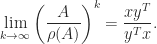
 (since
  ).
). . If
. If  and Theorem 4 says that
  . We illustrate this result in MATLAB using a scaled magic square matrix.
 , as
, as  is the rank-
 , and it is also rank-
 , as in this case every column is a multiple of the vector with alternating elements
  . For
. For  ,
,  is nonsingular and the inverse is the tridiagonal (but not Toeplitz) matrix
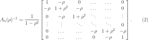
 ,
,  is positive definite, since every leading principal submatrix has positive determinant, as can also be seen by noting that the inverse is diagonally dominant with positive diagonal, so that
  is positive definite and hence
  ,
,  ,
,  , we know that
  with
with 
 for
for  .
. continues to hold with
  replaced by
  .
.
 permutations
  ) of the sequence
  and
and  is the number of inversions in
  , that is, the number of pairs
  with
with  . Each term in the sum is a signed product of
  .
.

 , where
  denotes the
  submatrix of
  for a scalar
  . This formula is called the expansion by minors because
  is a minor of
  is triangular then
  . If
. If  is unitary then
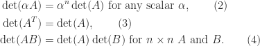
  on using (3) and (4). An
  of
of  . Since the eigenvalues are the roots of the characteristic polynomial
  , this relation follows by setting
  in the expression
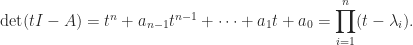
 , the determinant is
 the determinant is tedious to write down. If one must compute
  . As this expression indicates, the determinant is prone to overflow and underflow in floating-point arithmetic, so it may be preferable to compute
  .
.
 is the
  element
  ). More generally, Cramer’s rule says that the components of the solution to a linear system
  are given by
 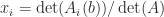 , where
  denotes
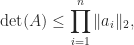
  is Hadamard’s inequality. Note that for such
  ,
,  is real and positive (being the product of the eigenvalues, which are real and positive) and the diagonal elements are also real and positive (since
  ).
).
 or by using a QR factorization of
 ![A = [a_1,a_2,\dots,a_n] \in\mathbb{C}^{n\times n}](https://s0.wp.com/latex.php?latex=A+%3D+%5Ba_1%2Ca_2%2C%5Cdots%2Ca_n%5D+%5Cin%5Cmathbb%7BC%7D%5E%7Bn%5Ctimes+n%7D&bg=ffffff&fg=222222&s=0&c=20201002) ,
,
 , whose sides are the columns of
  . It might be tempting to use
  as a measure of how close a nonsingular matrix
  can be given any value by a suitable choice of
  is perfectly conditioned:
  , where
 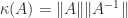 is the condition number.
 and
and  if and only if the columns of
  the Hadamard condition number. In general,
  , but if
  (Higham, 2002, Prob. 14.13). Dixon (1984) shows that for classes of
 , so
, so  for large
  , where
  denotes the mean value. This MATLAB example illustrates these points.
 term is the permanent. The permanent arises in combinatorics and quantum mechanics and is much harder to compute than the determinant: no algorithm is known for computing the permanent in
  operations for a polynomial
  , …,
, …,  by
by
 of degree at most
  , that is,
  ,
, 
![a = [a_1,a_2,\dots,a_n]^T](https://s0.wp.com/latex.php?latex=a+%3D+%5Ba_1%2Ca_2%2C%5Cdots%2Ca_n%5D%5ET&bg=ffffff&fg=222222&s=0&c=20201002) is the vector of coefficients. This is known as the dual problem. We know from polynomial interpolation theory that there is a unique interpolant if the
is the vector of coefficients. This is known as the dual problem. We know from polynomial interpolation theory that there is a unique interpolant if the 
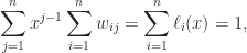
 find weights
  such that
  ,
,  for some
  then
then  . Consequently, we have
 in the
  contains a term
  (from the main diagonal), so
  . Hence
 . Equating elements in the
  gives
gives
 is the Kronecker delta (equal to
  and
and  takes the value
  and
and  ,
,  . It is not hard to see that this polynomial is the Lagrange basis polynomial:
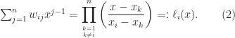

 denotes the sum of all distinct products of
  (that is,
  is the
  and
and  has a checkerboard sign pattern: the
  .
.
 is a degree
 and
and  .
. and
and ![\notag V = \left[\begin{array}{ccccc} 1 & 1 & 1 & 1 & 1\\ 0 & \frac{1}{4} & \frac{1}{2} & \frac{3}{4} & 1\\[\smallskipamount] 0 & \frac{1}{16} & \frac{1}{4} & \frac{9}{16} & 1\\[\smallskipamount] 0 & \frac{1}{64} & \frac{1}{8} & \frac{27}{64} & 1\\[\smallskipamount] 0 & \frac{1}{256} & \frac{1}{16} & \frac{81}{256} & 1 \end{array}\right], \quad V^{-1} = \left[\begin{array}{ccccc} 1 & -\frac{25}{3} & \frac{70}{3} & -\frac{80}{3} & \frac{32}{3}\\[\smallskipamount] 0 & 16 & -\frac{208}{3} & 96 & -\frac{128}{3}\\ 0 & -12 & 76 & -128 & 64\\[\smallskipamount] 0 & \frac{16}{3} & -\frac{112}{3} & \frac{224}{3} & -\frac{128}{3}\\[\smallskipamount] 0 & -1 & \frac{22}{3} & -16 & \frac{32}{3} \end{array}\right],](https://s0.wp.com/latex.php?latex=%5Cnotag+V+%3D+%5Cleft%5B%5Cbegin%7Barray%7D%7Bccccc%7D+1+%26+1+%26+1+%26+1+%26+1%5C%5C+0+%26+%5Cfrac%7B1%7D%7B4%7D+%26+%5Cfrac%7B1%7D%7B2%7D+%26+%5Cfrac%7B3%7D%7B4%7D+%26+1%5C%5C%5B%5Csmallskipamount%5D+0+%26+%5Cfrac%7B1%7D%7B16%7D+%26+%5Cfrac%7B1%7D%7B4%7D+%26+%5Cfrac%7B9%7D%7B16%7D+%26+1%5C%5C%5B%5Csmallskipamount%5D+0+%26+%5Cfrac%7B1%7D%7B64%7D+%26+%5Cfrac%7B1%7D%7B8%7D+%26+%5Cfrac%7B27%7D%7B64%7D+%26+1%5C%5C%5B%5Csmallskipamount%5D+0+%26+%5Cfrac%7B1%7D%7B256%7D+%26+%5Cfrac%7B1%7D%7B16%7D+%26+%5Cfrac%7B81%7D%7B256%7D+%26+1+%5Cend%7Barray%7D%5Cright%5D%2C+%5Cquad+V%5E%7B-1%7D+%3D+%5Cleft%5B%5Cbegin%7Barray%7D%7Bccccc%7D+1+%26+-%5Cfrac%7B25%7D%7B3%7D+%26+%5Cfrac%7B70%7D%7B3%7D+%26+-%5Cfrac%7B80%7D%7B3%7D+%26+%5Cfrac%7B32%7D%7B3%7D%5C%5C%5B%5Csmallskipamount%5D+0+%26+16+%26+-%5Cfrac%7B208%7D%7B3%7D+%26+96+%26+-%5Cfrac%7B128%7D%7B3%7D%5C%5C+0+%26+-12+%26+76+%26+-128+%26+64%5C%5C%5B%5Csmallskipamount%5D+0+%26+%5Cfrac%7B16%7D%7B3%7D+%26+-%5Cfrac%7B112%7D%7B3%7D+%26+%5Cfrac%7B224%7D%7B3%7D+%26+-%5Cfrac%7B128%7D%7B3%7D%5C%5C%5B%5Csmallskipamount%5D+0+%26+-1+%26+%5Cfrac%7B22%7D%7B3%7D+%26+-16+%26+%5Cfrac%7B32%7D%7B3%7D+%5Cend%7Barray%7D%5Cright%5D%2C+&bg=ffffff&fg=222222&s=0&c=20201002)
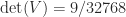 .
. satisfies
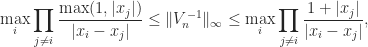
 for all
  for all
  . It is also known that for any set of real points
 we have
  , where the lower bound is an extremely fast growing function of the dimension!
 of Björck and Pereyra (1970). There is now a long list of generalizations of this algorithm in various directions, including for confluent Vandermonde-like matrices (Higham, 1990), as well as for more specialized problems (Demmel and Koev, 2005) and more general ones (Bella et al., 2009). Another important observation is that the exponential lower bounds are for real nodes. For complex nodes
  can be much better conditioned. Indeed when the
  is the unitary Fourier matrix and so
  we obtain
 in the case of (4)).
 with
with  having degree
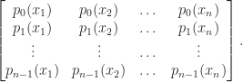
 . This little matrix has been used as an example and for test purposes in many research papers and books over the years, in particular by John Todd, who described it as “the notorious matrix
  of T. S. Wilson”.
 for a “positive definite symmetric
  ” and he gave the positive definite matrix
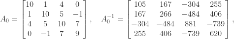
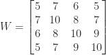
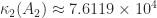
 . The matrix
  is therefore a factor 12 more ill conditioned than
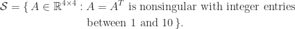
 and found that about 0.21 percent of them had a larger condition number than
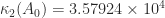
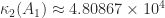 . How far is this matrix from being a worst case?
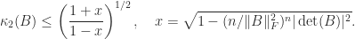
 for
for  . It is possible to obtain a bound from first principles by using the relation
  since
since  ,
,
 , using the fact that
  is monotonically increasing for
  , gives
 ,
,
 , since
  we have
  , and hence
 . The bounds (1) and (2) remain valid if we modify the definitions of
  to allow zero elements (note that Rutishauser’s matrix
  elements. Exhaustively searching over the sets in reasonable time is possible with a carefully optimized code. Higham and Lettington (2021) use a MATLAB code that loops over all symmetric matrices with integer elements between
  (since
 . and determinant
  . The maximum over
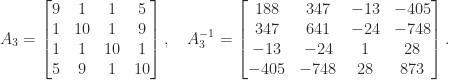
 and determinant


![\notag R = \begin{bmatrix} \sqrt{5} & \frac{7\,\sqrt{5}}{5} & \frac{6\,\sqrt{5}}{5} & \sqrt{5}\\[\smallskipamount] 0 & \frac{\sqrt{5}}{5} & -\frac{2\,\sqrt{5}}{5} & 0\\[\smallskipamount] 0 & 0 & \sqrt{2} & \frac{3\,\sqrt{2}}{2}\\[\smallskipamount] 0 & 0 & 0 & \frac{\sqrt{2}}{2} \end{bmatrix} \quad (W = R^TR).](https://s0.wp.com/latex.php?latex=%5Cnotag+R+%3D+%5Cbegin%7Bbmatrix%7D+%5Csqrt%7B5%7D+%26+%5Cfrac%7B7%5C%2C%5Csqrt%7B5%7D%7D%7B5%7D+%26+%5Cfrac%7B6%5C%2C%5Csqrt%7B5%7D%7D%7B5%7D+%26+%5Csqrt%7B5%7D%5C%5C%5B%5Csmallskipamount%5D+0+%26+%5Cfrac%7B%5Csqrt%7B5%7D%7D%7B5%7D+%26+-%5Cfrac%7B2%5C%2C%5Csqrt%7B5%7D%7D%7B5%7D+%26+0%5C%5C%5B%5Csmallskipamount%5D+0+%26+0+%26+%5Csqrt%7B2%7D+%26+%5Cfrac%7B3%5C%2C%5Csqrt%7B2%7D%7D%7B2%7D%5C%5C%5B%5Csmallskipamount%5D+0+%26+0+%26+0+%26+%5Cfrac%7B%5Csqrt%7B2%7D%7D%7B2%7D+%5Cend%7Bbmatrix%7D+%5Cquad+%28W+%3D+R%5ETR%29.+&bg=ffffff&fg=222222&s=0&c=20201002)
 element, it is unremarkable. If we factor out the diagonal then we obtain the
  factorization, which has rational elements:
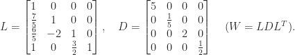
 with a
  matrix
  with
with  , but examples are known for
  for which the factorization does not exist. This result is mentioned by Taussky (1961) and goes back to Hermite, Minkowski, and Mordell. Higham and Lettington (2021) found the integer factor
 it is necessary that a certain quadratic equation in
 and two rational factors:
![\notag Z_1=\left[ \begin{array}{cccc} \frac{1}{2} & 1 & 0 & 1 \\ \frac{3}{2} & 2 & 3 & 3 \\ \frac{1}{2} & 1 & 0 & 0 \\ \frac{3}{2} & 2 & 1 & 0 \\ \end{array} \right], \quad Z_2=\left[ \begin{array}{@{\mskip2mu}rrrr} \frac{3}{2} & 2 & 2 & 2 \\ \frac{3}{2} & 2 & 2 & 1 \\ \frac{1}{2} & 1 & 1 & 2 \\ -\frac{1}{2} & -1 & 1 & 1 \\ \end{array} \right].](https://s0.wp.com/latex.php?latex=%5Cnotag+Z_1%3D%5Cleft%5B+%5Cbegin%7Barray%7D%7Bcccc%7D++%5Cfrac%7B1%7D%7B2%7D+%26+1+%26+0+%26+1+%5C%5C++%5Cfrac%7B3%7D%7B2%7D+%26+2+%26+3+%26+3+%5C%5C++%5Cfrac%7B1%7D%7B2%7D+%26+1+%26+0+%26+0+%5C%5C++%5Cfrac%7B3%7D%7B2%7D+%26+2+%26+1+%26+0+%5C%5C+%5Cend%7Barray%7D+%5Cright%5D%2C+%5Cquad+Z_2%3D%5Cleft%5B+%5Cbegin%7Barray%7D%7B%40%7B%5Cmskip2mu%7Drrrr%7D++%5Cfrac%7B3%7D%7B2%7D+%26+2+%26+2+%26+2+%5C%5C++%5Cfrac%7B3%7D%7B2%7D+%26+2+%26+2+%26+1+%5C%5C++%5Cfrac%7B1%7D%7B2%7D+%26+1+%26+1+%26+2+%5C%5C++-%5Cfrac%7B1%7D%7B2%7D+%26+-1+%26+1+%26+1+%5C%5C+%5Cend%7Barray%7D+%5Cright%5D.+&bg=ffffff&fg=222222&s=0&c=20201002)
 of
of  (a problem also considered in Higham, Lettington, and Schmidt (2021)), with integer