An circulant matrix is defined by parameters, the elements in the first row, and each subsequent row is a cyclic shift forward of the one above:

Circulant matrices have the important property that they are diagonalized by the discrete Fourier transform matrix

which satisfies , so that is a unitary matrix. ( is a Vandermonde matrix with points the roots of unity.) Specifically,

Hence circulant matrices are normal (). Moreover, the eigenvalues are given by , where is the first unit vector.

Note that one particular eigenpair is immediate, since , where is the vector of ones.

The factorization (1) enables a circulant linear system to be solved in flops, since multiplication by can be done using the fast Fourier transform.

A particular circulant matrix is the (up) shift matrix , the version of which is

It is not hard to see that

Since powers of commute, it follows that any two circulant matrices commute (this is also clear from (1)). Furthermore, the sum and product of two circulant matrices is a circulant matrix and the inverse of a nonsingular circulant matrix is a circulant matrix.

One important use of circulant matrices is to act as preconditioners for Toeplitz linear systems. Several methods have been proposed for constructing a circulant matrix from a Toeplitz matrix, including copying the central diagonals and wrapping them around and finding the nearest circulant matrix to the Toeplitz matrix. See Chan and Ng (1996) or Chan and Jin (2017) for a summary of work on circulant preconditioners for Toeplitz systems.

An interesting circulant matrix is anymatrix('core/circul_binom',n) in the Anymatrix collection, which is the circulant matrix whose first row has th element . The eigenvalues are , , where . The matrix is singular when is a multiple of 6, in which case the null space has dimension 2. Example:

>> n = 6; C = anymatrix('core/circul_binom',n), svd(C)
C =
     1     6    15    20    15     6
     6     1     6    15    20    15
    15     6     1     6    15    20
    20    15     6     1     6    15
    15    20    15     6     1     6
     6    15    20    15     6     1
ans =
   6.3000e+01
   2.8000e+01
   2.8000e+01
   1.0000e+00
   2.0244e-15
   7.6607e-16

The definition of matrix multiplication says that for matrices and , the product is given by . Each element of is an inner product of a row of and a column of , so if this formula is used then the cost of forming is additions and multiplications, that is, operations. For over a century after the development of matrix algebra in the 1850s by Cayley, Sylvester and others, all methods for matrix multiplication were based on this formula and required operations.

In 1969 Volker Strassen showed that when the product can be computed from the formulas

The evaluation requires multiplications and additions instead of multiplications and additions for the usual formulas.

At first sight, Strassen’s formulas may appear simply to be a curiosity. However, the formulas do not rely on commutativity so are valid when the and are matrices, in which case for large dimensions the saving of one multiplication greatly outweighs the extra additions. Assuming is a power of , we can partition and into four blocks of size , apply Strassen’s formulas for the multiplication, and then apply the same formulas recursively on the half-sized matrix products.

Let us examine the number of multiplications for the recursive Strassen algorithm. Denote by the number of scalar multiplications required to multiply two matrices. We have , so

But . The number of additions can be shown to be of the same order of magnitude, so the algorithm requires operations.

Strassen’s work sparked interest in finding matrix multiplication algorithms of even lower complexity. Since there are elements of data, which must each participate in at least one operation, the exponent of in the operation count must be at least .

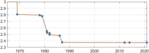
The current record upper bound on the exponent is , proved by Alman and Vassilevska Williams (2021) which improved on the previous record of , proved by Le Gall (2014) The following figure plots the best upper bound for the exponent for matrix multiplication over time.

In the methods that achieve exponents lower than 2.775, various intricate techniques are used, based on representing matrix multiplication in terms of bilinear or trilinear forms and their representation as tensors having low rank. Laderman, Pan, and Sha (1993) explain that for these methods “very large overhead constants are hidden in the `‘ notation”, and that the methods “improve on Strassen’s (and even the classical) algorithm only for immense numbers .”

Strassen’s method, when carefully implemented, can be faster than conventional matrix multiplication for reasonable dimensions. In practice, one does not recur down to matrices, but rather uses conventional multiplication once matrices are reached, where the parameter is tuned for the best performance.

Strassen’s method has the drawback that it satisfies a weaker form of rounding error bound that conventional multiplication. For conventional multiplication of and we have the componentwise bound

where and is the unit roundoff. For Strassen’s method we have only a normwise error bound. The following result uses the norm , which is not a consistent norm.

Theorem 1 (Brent). Let , where . Suppose that is computed by Strassen’s method and that is the threshold at which conventional multiplication is used. The computed product satisfies

With full recursion () the constant in (2) is , whereas with just one level of recursion () it is . These compare with for conventional multiplication (obtained by taking norms in (1)). So the constant for Strassen’s method grows at a faster rate than that for conventional multiplication no matter what the choice of .

The fact that Strassen’s method does not satisfy a componentwise error bound is a significant weakness of the method. Indeed Strassen’s method cannot even accurately multiply by the identity matrix. The product

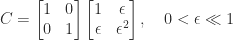
is evaluated exactly in floating-point arithmetic by conventional multiplication, but Strassen’s method computes

Because involves subterms of order unity, the error will be of order . Thus the relative error ,

Another weakness of Strassen’s method is that while the scaling , where is diagonal, leaves (1) unchanged, it can alter (2) by an arbitrary amount. Dumitrescu (1998) suggests computing , where the diagonal matrices and are chosen to equilibrate the rows of and the columns of in the -norm; he shows that this scaling can improve the accuracy of the result. Further investigations along these lines are made by Ballard et al. (2016).

Should one use Strassen’s method in practice, assuming that an implementation is available that is faster than conventional multiplication? Not if one needs a componentwise error bound, which ensures accurate products of matrices with nonnegative entries and ensures that the column scaling of and row scaling of has no effect on the error. But if a normwise error bound with a faster growing constant than for conventional multiplication is acceptable then the method is worth considering.

References

This is a minimal set of references, which contain further useful references within.
- Josh Alman and Virginia Vassilevska Williams. A refined laser method and faster matrix multiplication. In Proceedings of the 2021 ACM-SIAM Symposium on Discrete Algorithms (SODA), Society for Industrial and Applied Mathematics, January 2021, pages 522–539.
- Grey Ballard, Austin R. Benson, Alex Druinsky, Benjamin Lipshitz, and Oded Schwartz. Improving the numerical stability of fast matrix multiplication. SIAM J. Matrix Anal. Appl, 37(4):1382–1418, 2016.
- Benson, Alex Druinsky, Benjamin Lipshitz, and Oded Schwartz. Improving the numerical stability of fast matrix multiplication. SIAM J. Matrix Anal. Appl., 37(4):1382–1418, 2016.
- Dario A. Bini. Fast matrix multiplication. In Handbook of Linear Algebra, Leslie Hogben, editor, second edition, Chapman and Hall/CRC, Boca Raton, FL, USA, 2014, pages 61.1–61.17.
- Bogdan Dumitrescu. Improving and estimating the accuracy of Strassen’s algorithm. Numer. Math., 79:485–499, 1998.
- Nicholas J. Higham, Accuracy and Stability of Numerical Algorithms, second edition, Society for Industrial and Applied Mathematics, Philadelphia, PA, USA, 2002.
- Jianyu Huang, Tyler M. Smith, Greg M. Henry, and Robert A. van de Geijn. Strassen’s algorithm reloaded. In SC16: International Conference for High Performance Computing, Networking, Storage and Analysis, IEEE, November 2016.
- Jianyu Huang, Chenhan D. Yu, and Robert A. van de Geijn. Strassen’s algorithm reloaded on GPUs, ACM Trans. Math. Software, 46(1):1:1–1:22, 2020.
- Julian Laderman, Victor Pan, and Xuan-He Sha. On practical algorithms for accelerated matrix multiplication. Linear Algebra Appl., 162–164:557–588, 1992.
- François Le Gall. Powers of tensors and fast matrix multiplication. In Proceedings of the 39th International Symposium on Symbolic and Algebraic Computation, 2014, pages 296–303.
This article is part of the “What Is” series, available from https://nhigham.com/category/what-is and in PDF form from the GitHub repository https://github.com/higham/what-is.