Matrix rank is an important concept in linear algebra. While rank deficiency can be a sign of an incompletely or improperly specified problem (a singular system of linear equations, for example), in some problems low rank of a matrix is a desired property or outcome. Here we present some fundamental rank relations in a concise form useful for reference. These are all immediate consequences of the singular value decomposition (SVD), but we give elementary (albeit not entirely self-contained) proofs of them.
The rank of a matrix 


A rank-


Each column of 


Here are some fundamental rank equalities and inequalities.
Rank-Nullity Theorem
The rank-nullity theorem says that

where 
Rank Bound
The rank cannot exceed the number of columns, or, by (5) below, the number of rows:

Rank of a Sum
For any 

The upper bound follows from the fact that the dimension of the sum of two subspaces cannot exceed the sum of the dimensions of the subspaces. Interestingly, the upper bound is also a corollary of the bound (3) for the rank of a matrix product, because
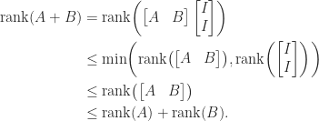
For the lower bound, writing 

Rank of and 
For any

Indeed 


Rank of a General Product
For any 

If ![B = [b_1,\dots,b_n]](https://s0.wp.com/latex.php?latex=B+%3D+%5Bb_1%2C%5Cdots%2Cb_n%5D&bg=ffffff&fg=222222&s=0&c=20201002)
![AB = [Ab_1,\dots,Ab_n]](https://s0.wp.com/latex.php?latex=AB+%3D+%5BAb_1%2C%5Cdots%2CAb_n%5D&bg=ffffff&fg=222222&s=0&c=20201002)

The latter inequality can be proved without using (5) (our proof of which uses (3)), as follows. Suppose 


Rank of a Product of Full-Rank Matrices
We have

We note that 


and hence 
Another important relation is

This is a consequence of the equality 
Ranks of and 
By (2) and (3) we have 


In other words, the rank of
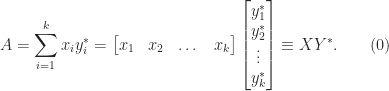
Full-Rank Factorization


![Y = [y_1,y_2,\dots, y_n]](https://s0.wp.com/latex.php?latex=Y+%3D+%5By_1%2Cy_2%2C%5Cdots%2C+y_n%5D&bg=ffffff&fg=222222&s=0&c=20201002)


Rank and Minors
A characterization of rank that is sometimes used as the definition is that it is the size of the largest nonsingular square submatrix. Equivalently, the rank is the size of the largest nonzero minor, where a minor of size 
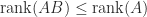
rank(AB) and rank(BA)
Although 


Note that 


How to Find Rank
If we have a full-rank factorization of

where 


In floating-point arithmetic, the standard algorithms for computing the SVD are numerically stable, that is, the computed singular values are the exact singular values of a matrix 


>> n = 4; A = zeros(n); A(:) = 1:n^2, svd(A)
A =
     1     5     9    13
     2     6    10    14
     3     7    11    15
     4     8    12    16
ans =
   3.8623e+01
   2.0713e+00
   1.5326e-15
   1.3459e-16
The matrix has rank 

rank function computes the rank as the number of singular values exceeding 

References
An excellent reference for further rank relations is Horn and Johnson. Stewart describes some of the issues associated with rank-deficient matrices in practical computation.
- Roger A. Horn and Charles R. Johnson, Matrix Analysis, second edition, Cambridge University Press, 2013. My review of the second edition.
- G. W. Stewart, Rank Degeneracy, SIAM J. Sci. Statist. Comput. 5 (2), 403–413, 1984
 such that
 needs to make any negative eigenvalues of
  and assume that
  .
. ,
,  has eigenvalues
  , and so the smallest possible
  is
is  . This choice of
  , so that each diagonal entry undergoes a relative perturbation of size
  . Write
  and note that
  is symmetric with unit diagonal. Then
 is positive semidefinite if and only if
  is positive semidefinite, the smallest possible
  .
. as
as  independent variables and ask for the solution of the optimization problem
 (since
  and
and  .
. is positive semidefinite then from standard eigenvalue inequalities,

 satisfies the constraints of
  , this means that this
  -norm, though the solution is obviously not unique in general.
 such that
  for an upper triangular
  with positive diagonal elements, so that
  is positive definite. The methods of Gill, Murray, and Wright (1981) and Schnabel and Eskow (1990) compute a diagonal
  ) flops), so this approach is likely to require fewer flops than computing the minimum eigenvalue or solving an optimization problem, but the perturbations produces will not be optimal.
 Fiedler matrix
 , so
, so  . The Gill–Murray–Wright method gives
  with diagonal elements
 while the Schnabel–Eskow method gives
  with diagonal elements
 . If we increase the diagonal elements of
  by 0.5 to give comparable smallest eigenvalues for the perturbed matrices then we have

 symmetric positive definite matrix
  to be the matrix resulting from adding
  to the
  and
and  elements and we ask when is
 has rank
  ,
,  repeated
  times. Hence we can write
  , where
  and
and  . Adding
  to
to  decreases or leaves unchanged each eigenvalue. However, more is true: after each of these rank-
 , we have (Horn and Johnson, Cor. 4.3.7)
 , so
, so  is the product of the eigenvalues of
  .
.
 . Hence the condition for

 for
for
 .
. is set to zero is
  , or equivalently
  . To check either of these conditions we need just
  ,
,  , and
, and  . These elements can be computed without computing the whole inverse by solving the equations
  for
for  , for the
  of
of  Lehmer matrix, which has
  for
for  :
:![\notag A = \begin{bmatrix} 1 & \frac{1}{2} & \frac{1}{3} & \frac{1}{4} \\[3pt] \frac{1}{2} & 1 & \frac{2}{3} & \frac{1}{2} \\[3pt] \frac{1}{3} & \frac{2}{3} & 1 & \frac{3}{4} \\[3pt] \frac{1}{4} & \frac{1}{2} & \frac{3}{4} & 1 \end{bmatrix}.](https://s0.wp.com/latex.php?latex=%5Cnotag+++A+%3D+%5Cbegin%7Bbmatrix%7D+++++++++1+++++++++++%26+%5Cfrac%7B1%7D%7B2%7D++%26+%5Cfrac%7B1%7D%7B3%7D+%26+%5Cfrac%7B1%7D%7B4%7D+%5C%5C%5B3pt%5D+++++++++%5Cfrac%7B1%7D%7B2%7D+%26+++++++++++1++%26+%5Cfrac%7B2%7D%7B3%7D+%26+%5Cfrac%7B1%7D%7B2%7D+%5C%5C%5B3pt%5D+++++++++%5Cfrac%7B1%7D%7B3%7D+%26++%5Cfrac%7B2%7D%7B3%7D+%26+1+++++++++++%26+%5Cfrac%7B3%7D%7B4%7D+%5C%5C%5B3pt%5D+++++++++%5Cfrac%7B1%7D%7B4%7D+%26++%5Cfrac%7B1%7D%7B2%7D+%26+%5Cfrac%7B3%7D%7B4%7D+%26++1+++++++++%5Cend%7Bbmatrix%7D.+&bg=ffffff&fg=222222&s=0&c=20201002)
 . Any off-diagonal element except the
  element can be zeroed without destroying positive definiteness, and if the
  . For
. For  and
and  , the following plot shows in red
  and in blue
  ; the black dots are the endpoints of the closure of the interval
  and the vertical black line is the value
  . Clearly,
  , which is why zeroing this element causes a loss of positive definiteness. Note that
  to any number less than
  without losing definiteness.
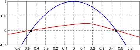
 of elements to be modified we may wish to determine subsets (including a maximal subset) of
  on the smallest eigenvalue, which corresponds to another projection. Both these projections are supported in the algorithm of Higham and Strabić (2016), implemented in the code at
  is (to four significant figures)
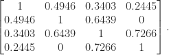
 -Factorizations with Small Pivots
 is unitarily invariant if
 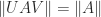 for all unitary
  and
and  and for all
  and
and  , using the fact that
  , we obtain
 ,
,

 , so
, so  depends only on the singular values. Indeed, for the 2-norm and the Frobenius norm we have
  and
and  . Here, and throughout this article,
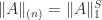
  . Another implication of the singular value dependence is that
  for all
  such that
  is an absolute norm on
  and
and  for any permutation matrix
  and all
  for all
  implies
  for all
  for all
  are the singular values of
  -norm, obtaining the class of Schatten
 , which is called the trace norm or nuclear norm. It can act as a proxy for the rank of a matrix. The trace norm can be expressed as
  , where
  is a polar decomposition.
 and
and  .
. , the matrix
  is the
  (
( ), the unitary polar factor is the
  have SVDs with diagonal matrices
  , where the diagonal elements are arranged in nonincreasing order. Then
  for every unitarily invariant norm.
 for which the product
  is defined,
 for all
  if and only if
  for all
  for all
  if and only if the norm is a positive scalar multiple of the Frobenius norm.