Let  be an upper triangular matrix. The upper bounds for
  that we will discuss depend only on the absolute values of the elements of
  . This limits the ability of the bounds to distinguish between well-conditioned and ill-conditioned matrices. For example, consider
![\notag \begin{gathered} T_1 = \left[\begin{array}{crrrr} 1 & -2 & -2 & -2 & -2\\ & 1 & -2 & -2 & -2\\ & & 1 & -2 & -2\\ & & & 1 & -2\\ & & & & 1 \end{array}\right], \quad T_1^{-1} = \left[\begin{array}{ccccc} 1 & 2 & 6 & 18 & 54\\ & 1 & 2 & 6 & 18\\ & & 1 & 2 & 6\\ & & & 1 & 2\\ & & & & 1 \end{array}\right], \\ T_2 = \left[\begin{array}{ccccc} 1 & 2 & 2 & 2 & 2\\ & 1 & 2 & 2 & 2\\ & & 1 & 2 & 2\\ & & & 1 & 2\\ & & & & 1 \end{array}\right], \quad T_2^{-1} = \left[\begin{array}{crrrr} 1 & -2 & 2 & -2 & 2\\ & 1 & -2 & 2 & -2\\ & & 1 & -2 & 2\\ & & & 1 & -2\\ & & & & 1 \end{array}\right]. \end{gathered}](https://s0.wp.com/latex.php?latex=%5Cnotag+%5Cbegin%7Bgathered%7D++++++T_1+%3D+++++++%5Cleft%5B%5Cbegin%7Barray%7D%7Bcrrrr%7D+1+%26+-2+%26+-2+%26+-2+%26+-2%5C%5C+++++++++%26+1+%26+-2+%26+-2+%26+-2%5C%5C+++++++++%26+++%26+1+%26+-2+%26+-2%5C%5C+++++++++%26+++%26+++%26+1+%26+-2%5C%5C+++++++++%26+++%26+++%26+++%26+1+%5Cend%7Barray%7D%5Cright%5D%2C+%5Cquad++++++T_1%5E%7B-1%7D+%3D++++++%5Cleft%5B%5Cbegin%7Barray%7D%7Bccccc%7D++++++1+%26+2+%26+6+%26+18+%26+54%5C%5C++++++++%26+1+%26+2+%26+6+%26+18%5C%5C++++++++%26+++%26+1+%26+2+%26+6%5C%5C++++++++%26+++%26+++%26+1+%26+2%5C%5C++++++++%26+++%26+++%26+++%26+1++++++%5Cend%7Barray%7D%5Cright%5D%2C+%5C%5C+++++T_2+%3D+++++%5Cleft%5B%5Cbegin%7Barray%7D%7Bccccc%7D+++++1+%26+2+%26+2+%26+2+%26+2%5C%5C+++++++%26+1+%26+2+%26+2+%26+2%5C%5C+++++++%26+++%26+1+%26+2+%26+2%5C%5C+++++++%26+++%26+++%26+1+%26+2%5C%5C+++++++%26+++%26+++%26+++%26+1+++++%5Cend%7Barray%7D%5Cright%5D%2C+%5Cquad+++T_2%5E%7B-1%7D+%3D+++++%5Cleft%5B%5Cbegin%7Barray%7D%7Bcrrrr%7D++++++1+%26+-2+%26+2+%26+-2+%26+2%5C%5C++++++++%26+1+%26+-2+%26+2+%26+-2%5C%5C++++++++%26+++%26+1+%26+-2+%26+2%5C%5C++++++++%26+++%26+++%26+1+%26+-2%5C%5C++++++++%26+++%26+++%26+++%26+1+++++%5Cend%7Barray%7D%5Cright%5D.+%5Cend%7Bgathered%7D+&bg=ffffff&fg=222222&s=0&c=20201002)
The bounds for  and
and  will be the same, yet the inverses are of different sizes (the more so as the dimension increases).
Let  and write

where  is strictly upper triangular and hence nilpotent with
  . Then

Taking absolute values and using the triangle inequality gives

where the inequalities hold elementwise.
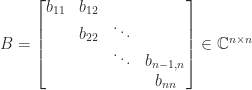
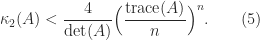
The comparison matrix  associated with a general
  is the matrix with
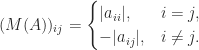
It is not hard to see that  is upper triangular with
  and so the bound (5) is
If we replace every element above the diagonal of by the most negative off-diagonal element in its row we obtain the upper triangular matrix  with
with

Then  , where
  , so
, so

Finally, let  , where
  is strictly upper triangular with every element above the diagonal equal to the maximum element of
  , that is,

Then

We note that , , and  are all nonsingular
  -matrices. We summarize the bounds.
Theorem 1.
If is a nonsingular upper triangular matrix then

We make two remarks.
- The bounds (6) are equally valid for lower triangular matrices as long as the maxima in the definitions of and are taken over columns instead of rows.
- We could equally well have written
 . The comparison matrix
  is unchanged, and (6) continues to hold as long as the maxima in the definitions of and are taken over columns rather than rows.
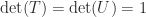
It follows from the theorem that

for the 1-, 2-, and  -norms and the Frobenius norm. Now , , and all have nonnegative inverses, and for a matrix
  with nonnegative inverse we have
  . Hence

where the big-Oh expressions show the asymptotic cost in flops of evaluating each term by solving the relevant triangular system. As the bounds become less expensive to compute they become weaker. The quantity  can be explicitly evaluated for
  , using
  . It has the same value for
  , and since
  we have

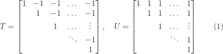
This bound is an equality for  for the matrix
  in (1).
For the Frobenius norm, evaluating  , and using
  , gives

For the  -norm, either of (7) and (8) can be the smaller bound depending on
  .
.
For the special case of a bidiagonal matrix  it is easy to show that
  , and so
  can be computed exactly in
  flops.
These upper bounds can be arbitrarily weak, even for a fixed  , as shown by the example

for which

As  ,
,  . On the other hand, the overestimation is bounded as a function of for triangular matrices resulting from certain pivoting strategies.
Theorem 1.
Suppose the upper triangular matrix satisfies
Then, for the  -, -, and -norms,

Proof. The first four inequalities are a combination of (3) and (6). The fifth inequality is obtained from the expression (7) for  with
with  .
.
Condition (9) is satisfied for the triangular factors from QR factorization with column pivoting and for the transpose of the unit lower triangular factors from LU factorization with any form of pivoting.
The upper bounds we have described have been derived independently by several authors, as explained by Higham (2002).


![\notag \begin{bmatrix} a & x & 0 & 0 \\ & b & y & 0 \\ & & c & z \\ & & & d \end{bmatrix}^{-1} = \begin{bmatrix} \frac{1}{a} & -\frac{x}{a\,b} & \frac{x\,y}{a\,b\,c} & -\frac{x\,y\,z}{a\,b\,c\,d} \\[3pt] & \frac{1}{b} & -\frac{y}{b\,c} & \frac{y\,z}{b\,c\,d} \\[3pt] & & \frac{1}{c} & -\frac{z}{c\,d} \\[3pt] & & & \frac{1}{d} \end{bmatrix}.](https://s0.wp.com/latex.php?latex=%5Cnotag+%5Cbegin%7Bbmatrix%7D+a+++++++++++%26+x+++++++++++++++%26+0++++++++++++++++++++%26+0+%5C%5C+++++++++++++%26+b+++++++++++++++%26+y++++++++++++++++++++%26+0+%5C%5C+++++++++++++%26+++++++++++++++++%26+c++++++++++++++++++++%26+z+%5C%5C+++++++++++++%26+++++++++++++++++%26++++++++++++++++++++++%26+d+%5Cend%7Bbmatrix%7D%5E%7B-1%7D+%3D+%5Cbegin%7Bbmatrix%7D+%5Cfrac%7B1%7D%7Ba%7D+%26+-%5Cfrac%7Bx%7D%7Ba%5C%2Cb%7D+%26+%5Cfrac%7Bx%5C%2Cy%7D%7Ba%5C%2Cb%5C%2Cc%7D+%26+-%5Cfrac%7Bx%5C%2Cy%5C%2Cz%7D%7Ba%5C%2Cb%5C%2Cc%5C%2Cd%7D+%5C%5C%5B3pt%5D+++++++++++++%26+%5Cfrac%7B1%7D%7Bb%7D+++++%26+-%5Cfrac%7By%7D%7Bb%5C%2Cc%7D++++++%26+%5Cfrac%7By%5C%2Cz%7D%7Bb%5C%2Cc%5C%2Cd%7D++++++++%5C%5C%5B3pt%5D+++++++++++++%26+++++++++++++++++%26+%5Cfrac%7B1%7D%7Bc%7D++++++++++%26+-%5Cfrac%7Bz%7D%7Bc%5C%2Cd%7D+++++++++++++%5C%5C%5B3pt%5D+++++++++++++%26+++++++++++++++++%26++++++++++++++++++++++%26+%5Cfrac%7B1%7D%7Bd%7D+%5Cend%7Bbmatrix%7D.+&bg=ffffff&fg=222222&s=0&c=20201002)
depend on
, as there is no cancellation in the formulas for
(less obvious, and provable by a scaling argument).
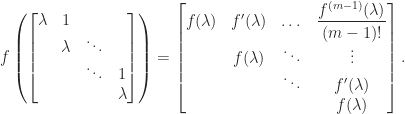
![f[\dots]](https://s0.wp.com/latex.php?latex=f%5B%5Cdots%5D&bg=ffffff&fg=222222&s=0&c=20201002)
is upper bidiagonal then
is upper triangular with
and
![\notag f_{ij} = b_{i,i+1} b_{i+1,i+2} \dots b_{j-1,j}\, f[b_{ii},b_{i+1,i+1}, \dots, b_{jj}], \quad j > i.](https://s0.wp.com/latex.php?latex=%5Cnotag+++++++f_%7Bij%7D+%3D+b_%7Bi%2Ci%2B1%7D+b_%7Bi%2B1%2Ci%2B2%7D+%5Cdots+b_%7Bj-1%2Cj%7D%5C%2C++++++++++++++++f%5Bb_%7Bii%7D%2Cb_%7Bi%2B1%2Ci%2B1%7D%2C+%5Cdots%2C+b_%7Bjj%7D%5D%2C+%5Cquad+j+%3E+i.+&bg=ffffff&fg=222222&s=0&c=20201002)


 of
of  , where
  is the matrix inverse. What is not always emphasized is that there are very few circumstances in which one should compute
  ) system
  by computing
  , but rather would carry out a division
  . In the
  case, it is faster and more accurate to solve a linear system by LU factorization (Gaussian elimination) with partial pivoting than by inverting
  , where
  matrix with
  , satisfies the normal equations
  . It is therefore natural to form the symmetric positive definite matrix
  and solve the normal equations by Cholesky factorization. While fast, this method is numerically unstable when
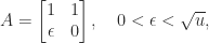
 is the unit roundoff of the floating point arithmetic, then
 , in floating-point arithmetic
  rounds to
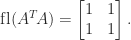
 has been lost.
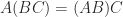 , and in general the cost of the evaluation of a product depends on where one puts the parentheses. One order may be much superior to others, so one should not simply evaluate the product in a fixed left-right or right-left order. For example, if
  ,
,  , and
, and  are
are  can be evaluated as
 : a vector outer product followed by a matrix–vector product, costing
  : a vector scalar product followed by a vector scaling, costing just
  in order to minimize the operation count is a
  ,
, for all
  ,
, factor is returned in the first argument, and it can be used to compute a direction of negative curvature (as needed in optimization), for example.
 that exploit the block structure and possible sparsity in
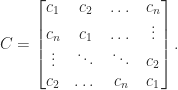
 in
in  operations, rather than the
  operations required if the circulant structure is ignored.
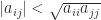
 indicates a matrix that is nearly singular. However, the size of
 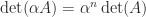 we can achieve any value for the determinant by multiplying by a scalar
  , yet
, yet  is no more or less nearly singular than
  .
.
 , yet
, yet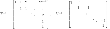
 element of
  then the matrix becomes singular! By contrast,
  for all
  , where the
  are the eigenvalue of
  , it follows that the matrix condition number
  is bounded below by the ratio of largest to smallest eigenvalue in absolute value, that is,

 is a singular value decomposition (SVD), with
  orthogonal and
  ,
,  . If
. If  and
and  are the same, but in general the eigenvalues
  can be very different.
 , and future exascale computer systems will be able to tackle even larger problems. Rounding error analysis shows that the computed solution satisfies a componentwise backward error bound that, under favorable assumptions, is of order
  , where
  for double precision and
  for single precision. This backward error bound cannot guarantee any stability for single precision solution of today’s largest problems and suggests a loss of half the digits in the backward error for double precision.
 for both half precision formats, suggesting a potentially complete loss of numerical stability. Yet inner products with
  of two
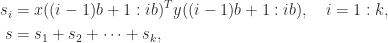
 and
and  is the block size. The inner product has been broken into
  smaller inner products of size
  , which are computed independently then summed. Many linear algebra algorithms are blocked in an analogous way, where the blocking is into submatrices with
  or
or  , so blocking brings a substantial reduction in the error bounds.
 . By computing the sum
  with a more accurate summation method the error constant is further reduced to
  (this is the FABsum method of Blanchard et al. (2020)).
 rather than
  for double precision, giving error bounds smaller by a factor up to
  .
. with one rounding error instead of two. This results in a reduction in error bounds by a factor
  , with matrices
  of fixed size, are available on Google tensor processing units, NVIDIA GPUs, and in the ARMv8-A architecture. For half precision inputs these devices can produce results of single precision quality, which can give a significant boost in accuracy when block FMAs are chained together to form a matrix product of arbitrary dimension.
 when a corresponding worst-case bound is proportional to
  , which is a significant reduction. Block FMAs and extended precision registers provide further reductions.
 solved in single precision with a block size of
  versus
  of a nonsingular matrix
  , for any matrix norm, where
  is the spectral radius (the largest magnitude of any eigenvalue of
 ), but it can be arbitrarily weak for nonnormal matrices.
 , where the
  are of similar order of magnitude.
 ,
,  .
. matrices with
  , generated by
  the formula (3) is prone to overflow, which can be avoided by evaluating it in higher precision arithmetic.
 ,
,  of
of  . We can rewrite this upper bound as
 larger than (4), this factor being attained for
  .
. then (4) reduces to
 , where
  and
and  (thus
(thus  is a correlation matrix), using
 using (6). For example, for the
  Pascal matrix
![\notag P_5 = \left[\begin{array}{ccccc} 1 & 1 & 1 & 1 & 1\\ 1 & 2 & 3 & 4 & 5\\ 1 & 3 & 6 & 10 & 15\\ 1 & 4 & 10 & 20 & 35\\ 1 & 5 & 15 & 35 & 70 \end{array}\right]](https://s0.wp.com/latex.php?latex=%5Cnotag+P_5+%3D+%5Cleft%5B%5Cbegin%7Barray%7D%7Bccccc%7D+1+%26+1+%26+1+%26+1+%26+1%5C%5C+1+%26+2+%26+3+%26+4+%26+5%5C%5C+1+%26+3+%26+6+%26+10+%26+15%5C%5C+1+%26+4+%26+10+%26+20+%26+35%5C%5C+1+%26+5+%26+15+%26+35+%26+70+%5Cend%7Barray%7D%5Cright%5D+&bg=ffffff&fg=222222&s=0&c=20201002)
 . The bounds from (4) and (5) are both
  , whereas combining (4) and (7) gives a bound of
  .
. for a matrix with integer entries. If a Cholesky, LU, or QR factorization of
  is easily computable, but in this case a good order of magnitude estimate of the condition number can be cheaply computed using condition estimation techniques (Higham, 2002, Chapter 15).
 symmetric matrices with integer elements bounded by
  ; see
; see  is a factorization
  , where
  and
and  are unitary and
  , with
  , where where
  . We sometimes write
  to specify the matrix to which the singular value belongs.
 or
or  , whose eigenvalues are the squares of the singular values of
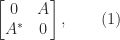
 zero eigenvalues if
  .
. ,
,
 .
.

 (the equality case in the Cauchy–Schwarz inequality). For example, (2) is equivalent to
 ,
,
 and nonsingular
  and
and  ,
,
 .
.
 . The bounds (5) and (6) are intuitively reasonable, because unitary transformations preserve singular values and the bounds quantify in different ways how close
  and
and  are to being unitary.
 , and
, and  . Then
 if
if  .
. is the leading principal submatrix of order
  ).
). and
and  . The first case is
  , so that
  and
and
 , so
, so  and
and
 . However, when
  may be less than the smallest singular value of
 ![A = [A_{11}~A_{12}]](https://s0.wp.com/latex.php?latex=A+%3D+%5BA_%7B11%7D%7EA_%7B12%7D%5D&bg=ffffff&fg=222222&s=0&c=20201002) then
then  for all
  is easy to compute or estimate. Here, we focus on triangular matrices. The bounds we derive can be applied to a general matrix if an LU or QR factorization is available.
 any matrix norm, and we take the consistency condition
  as one of the defining properties of a matrix norm.
![\notag \left[\begin{array}{crrrr} 1 & -\theta & -\theta & -\theta & -\theta\\ & 1 & -\theta & -\theta & -\theta\\ & & 1 & -\theta & -\theta\\ & & & 1 & -\theta\\ & & & & 1 \end{array}\right]^{-1} = \left[\begin{array}{ccccc} 1 & \theta & \theta(1+\theta) & \theta(1+\theta)^2 & \theta(1+\theta)^3\\ & 1 & \theta & \theta(1+\theta) & \theta(1+\theta)^2\\ & & 1 & \theta & \theta(1+\theta)\\ & & & 1 & \theta\\ & & & & 1 \end{array}\right]](https://s0.wp.com/latex.php?latex=%5Cnotag+++++++%5Cleft%5B%5Cbegin%7Barray%7D%7Bcrrrr%7D+++++++1+%26+-%5Ctheta+%26+-%5Ctheta+%26+-%5Ctheta+%26+-%5Ctheta%5C%5C+++++++++%26+1+%26+-%5Ctheta+%26+-%5Ctheta+%26+-%5Ctheta%5C%5C+++++++++%26+++%26+1+%26+-%5Ctheta+%26+-%5Ctheta%5C%5C+++++++++%26+++%26+++%26+1+%26+-%5Ctheta%5C%5C+++++++++%26+++%26+++%26+++%26+1+%5Cend%7Barray%7D%5Cright%5D%5E%7B-1%7D+%3D++++++%5Cleft%5B%5Cbegin%7Barray%7D%7Bccccc%7D++++++1+%26+%5Ctheta+%26+%5Ctheta%281%2B%5Ctheta%29+%26+%5Ctheta%281%2B%5Ctheta%29%5E2+%26+%5Ctheta%281%2B%5Ctheta%29%5E3%5C%5C++++++++%26+1+%26+%5Ctheta+%26+%5Ctheta%281%2B%5Ctheta%29+%26+%5Ctheta%281%2B%5Ctheta%29%5E2%5C%5C++++++++%26+++%26+1+%26+%5Ctheta+%26+%5Ctheta%281%2B%5Ctheta%29%5C%5C++++++++%26+++%26+++%26+1+%26+%5Ctheta%5C%5C++++++++%26+++%26+++%26+++%26+1++++++%5Cend%7Barray%7D%5Cright%5D+&bg=ffffff&fg=222222&s=0&c=20201002)


 be an eigenvalue with
  (the spectral radius) and
  , where
  is the vector of ones,
  , so
, so
 since
since  . Hence
 , whose eigenvalues are its diagonal entries
  , gives
 gives
gives
 , which yields another proof of (3) and (4).
 we have the lower bound
  . We can choose
  for
for  correct to within an order of magnitude.
 by repeated triangular solves, obtaining the lower bound
  . This bound is simply the power method applied to
  .
. exceeds
  . Note that in some references, such as Horn and Johnson (2013), the reverse ordering is used, with
  the largest eigenvalue. When it is necessary to specify what matrix
  is an eigenvalue of we write
  : the
: the  .
. is the quadratic form
  for
for  . As
. As  , where
  is unitary and
  . Then

 , respectively, This characterization of the extremal eigenvalues of
  is due to Lord Rayleigh (John William Strutt), and
  is called a Rayleigh quotient. The intermediate eigenvalues correspond to saddle points of
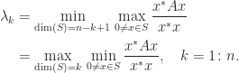
 are special cases of these characterizations.
 of Hermitian matrices. However, the Courant–Fischer theorem yields the upper and lower bounds


 and
and  ,
,
 . Inequality (3) with
  gives
gives
 , combined with (2), gives
 to the interval between two adjacent eigenvalues of
  , showing a possible configuration of the eigenvalues
  of
of  A specific example, in MATLAB, is
 and the trace is the sum of the eigenvalues, we can write
 are nonnegative and sum to
  , the norm of the perturbation, then most of the increase in the eigenvalues is concentrated in the largest, since (5) bounds how much the smaller eigenvalues can change:
 positive eigenvalues and
  negative eigenvalues then (3) with
  gives
gives
 gives
gives

 eigenvalues appear in one of these inequalities and
  appear in both. Therefore
  of the eigenvalues are equal to
  eigenvalues can differ from
  changes at most
  and
and  and so taking
  in (3) and
  in (4) gives
 .
.
 interlace those of
  for all
  interlace those of
  is given in the next result.
 in the formula
  that
that  for all
  . These relations are the first and last in a sequence of inequalities relating sums of eigenvalues to sums of diagonal elements obtained by Schur in 1923.
 is the set of diagonal elements of
  .
.![[\lambda_1,\dots,\lambda_n]](https://s0.wp.com/latex.php?latex=%5B%5Clambda_1%2C%5Cdots%2C%5Clambda_n%5D&bg=ffffff&fg=222222&s=0&c=20201002) of eigenvalues majorizes the ordered vector
of eigenvalues majorizes the ordered vector ![[\widetilde{a}_{11},\dots,\widetilde{a}_{nn}]](https://s0.wp.com/latex.php?latex=%5B%5Cwidetilde%7Ba%7D_%7B11%7D%2C%5Cdots%2C%5Cwidetilde%7Ba%7D_%7Bnn%7D%5D&bg=ffffff&fg=222222&s=0&c=20201002) of diagonal elements.
of diagonal elements.
 . Here is an illustration in MATLAB.
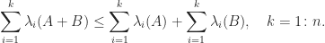
 , the inequality is the same as the upper bound of (1), and for
  it is an equality:
  .
. is a congruence transformation. Sylvester’s law of inertia says that congruence transformations preserve the inertia. A result of Ostrowski (1959) goes further by providing bounds on the ratios of the eigenvalues of the original and transformed matrices.
 and
and 
 .
. and so Ostrowski’s theorem reduces to the fact that a congruence with a unitary matrix is a similarity transformation and so preserves eigenvalues. The theorem shows that the further
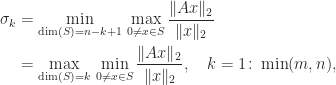
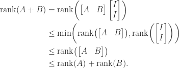
  is the maximum number of linearly independent columns, which is the dimension of the range space of
  . An important but non-obvious fact is that this is the same as the maximum number of linearly independent rows (see (5) below).
 , where
  . A sum of
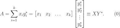
 ,
,  , …,
, …,  , so
, so  if
if  with
with 
 is the null space of

 and applying the upper bound gives
  , and likewise with the roles of
 implies
  , and
, and  , which implies
  is defined,
![B = [b_1,\dots,b_n]](https://s0.wp.com/latex.php?latex=B+%3D+%5Bb_1%2C%5Cdots%2Cb_n%5D&bg=ffffff&fg=222222&s=0&c=20201002) then
then ![AB = [Ab_1,\dots,Ab_n]](https://s0.wp.com/latex.php?latex=AB+%3D+%5BAb_1%2C%5Cdots%2CAb_n%5D&bg=ffffff&fg=222222&s=0&c=20201002) , so the columns of
, so the columns of  . Using (5) below, we then have
 . Let the columns of
  , so that
  for some matrix
  with
with  by the first part, so
  for some nonzero
  . But then
  , which contradicts the linear independence of the columns of
  .
.
 are both nonsingular
  matrices by (2), so their product has rank
 .
.
 for nonsingular
  . Interchanging the roles of
  and so
 has rank
  for some
  and
and  , both of rank
  by (4). Conversely, suppose that
  form a basis for the range space of
  such that
  ,
,  , and with
 ![Y = [y_1,y_2,\dots, y_n]](https://s0.wp.com/latex.php?latex=Y+%3D+%5By_1%2Cy_2%2C%5Cdots%2C+y_n%5D&bg=ffffff&fg=222222&s=0&c=20201002) we have
we have  . Finally,
  by (3), and since
  we have
  .
. submatrix.
 have some properties in common when both products are defined (notably they have the same nonzero eigenvalues),
  is not always equal to
  . A simple example is
  and
and  with
with  but
but  . An example with square
 and
and  , where
  ) and are useful for constructing examples.
 and
and  are orthogonal,
  . The rank of
  with
with  , where
  is a constant and
  . In general, we have no way to know whether tiny computed singular values signify exactly zero singular values. In practice, one typically defines a numerical rank based on a threshold and regards computed singular values less than the threshold as zero. Indeed the MATLAB
  , where
  is the largest computed singular value. If the data from which the matrix is constructed is uncertain then the definition of numerical rank should take into account the level of uncertainty in the data. Dealing with rank deficiency in the presence of data errors and in finite precision arithmetic is a tricky business.
 such that
 needs to make any negative eigenvalues of
  and assume that
  .
. ,
,  has eigenvalues
  , and so the smallest possible
  is
is  . This choice of
  , so that each diagonal entry undergoes a relative perturbation of size
  and note that
  is symmetric with unit diagonal. Then
 is positive semidefinite if and only if
  is positive semidefinite, the smallest possible
  .
. as
as 
 (since
  and
and  .
. is positive semidefinite then from standard eigenvalue inequalities,

 satisfies the constraints of
  , this means that this
  such that
  for an upper triangular
  is positive definite. The methods of Gill, Murray, and Wright (1981) and Schnabel and Eskow (1990) compute a diagonal
  ) flops), so this approach is likely to require fewer flops than computing the minimum eigenvalue or solving an optimization problem, but the perturbations produces will not be optimal.
 , so
, so  . The Gill–Murray–Wright method gives
  with diagonal elements
 while the Schnabel–Eskow method gives
  with diagonal elements
 . If we increase the diagonal elements of
  by 0.5 to give comparable smallest eigenvalues for the perturbed matrices then we have

 to be the matrix resulting from adding
  to the
  and
and  elements and we ask when is
 has rank
  ,
,  repeated
  times. Hence we can write
  , where
  and
and  . Adding
  to
to  decreases or leaves unchanged each eigenvalue. However, more is true: after each of these rank-
 , we have (Horn and Johnson, Cor. 4.3.7)
 , so
, so  is the product of the eigenvalues of
  .
.
 . Hence the condition for

 for
for
 .
. is set to zero is
  , or equivalently
  . To check either of these conditions we need just
  ,
,  , and
, and  . These elements can be computed without computing the whole inverse by solving the equations
  for
for  , for the
  of
of  for
for  :
:![\notag A = \begin{bmatrix} 1 & \frac{1}{2} & \frac{1}{3} & \frac{1}{4} \\[3pt] \frac{1}{2} & 1 & \frac{2}{3} & \frac{1}{2} \\[3pt] \frac{1}{3} & \frac{2}{3} & 1 & \frac{3}{4} \\[3pt] \frac{1}{4} & \frac{1}{2} & \frac{3}{4} & 1 \end{bmatrix}.](https://s0.wp.com/latex.php?latex=%5Cnotag+++A+%3D+%5Cbegin%7Bbmatrix%7D+++++++++1+++++++++++%26+%5Cfrac%7B1%7D%7B2%7D++%26+%5Cfrac%7B1%7D%7B3%7D+%26+%5Cfrac%7B1%7D%7B4%7D+%5C%5C%5B3pt%5D+++++++++%5Cfrac%7B1%7D%7B2%7D+%26+++++++++++1++%26+%5Cfrac%7B2%7D%7B3%7D+%26+%5Cfrac%7B1%7D%7B2%7D+%5C%5C%5B3pt%5D+++++++++%5Cfrac%7B1%7D%7B3%7D+%26++%5Cfrac%7B2%7D%7B3%7D+%26+1+++++++++++%26+%5Cfrac%7B3%7D%7B4%7D+%5C%5C%5B3pt%5D+++++++++%5Cfrac%7B1%7D%7B4%7D+%26++%5Cfrac%7B1%7D%7B2%7D+%26+%5Cfrac%7B3%7D%7B4%7D+%26++1+++++++++%5Cend%7Bbmatrix%7D.+&bg=ffffff&fg=222222&s=0&c=20201002)
 . Any off-diagonal element except the
  element can be zeroed without destroying positive definiteness, and if the
  . For
. For  and
and  , the following plot shows in red
  and in blue
  ; the black dots are the endpoints of the closure of the interval
  and the vertical black line is the value
  . Clearly,
  , which is why zeroing this element causes a loss of positive definiteness. Note that
  to any number less than
  without losing definiteness.
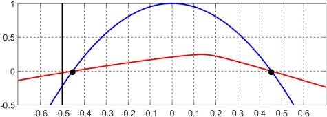
 of elements to be modified we may wish to determine subsets (including a maximal subset) of
  on the smallest eigenvalue, which corresponds to another projection. Both these projections are supported in the algorithm of Higham and Strabić (2016), implemented in the code at
  is (to four significant figures)
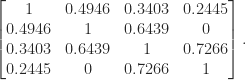
 -Factorizations with Small Pivots