An 


Here, 


for any consistent matrix norm:

Although the definition of an 


The concept of
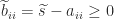
An immediate consequence of the definition is that the eigenvalues of an 


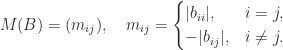
In fact, nonnegativity of the inverse characterizes

Theorem 1.
A nonsingular matrix
is an
.
Sometimes an
It is easy to check from the definitions, or using Theorem 1, that a triangular matrix 
![\notag T_4 = \left[\begin{array}{@{\mskip 5mu}c*{3}{@{\mskip 15mu} r}@{\mskip 5mu}} 1 & -1 & -1 & -1 \\ & 1 & -1 & -1 \\ & & 1 & -1 \\ & & & 1 \end{array}\right], \quad T_4^{-1} = \begin{bmatrix} 1 & 1 & 2 & 4\\ & 1 & 1 & 2\\ & & 1 & 1\\ & & & 1 \end{bmatrix}.](https://s0.wp.com/latex.php?latex=%5Cnotag+++++T_4+%3D+%5Cleft%5B%5Cbegin%7Barray%7D%7B%40%7B%5Cmskip+5mu%7Dc%2A%7B3%7D%7B%40%7B%5Cmskip+15mu%7D+r%7D%40%7B%5Cmskip+5mu%7D%7D++++++1+%26+++-1++%26++-1++%26+-1+%5C%5C++++++++%26++++1++%26++-1++%26+-1+%5C%5C++++++++%26+++++++%26+++1++%26+-1+%5C%5C++++++++%26+++++++%26++++++%26++1++++++++++++%5Cend%7Barray%7D%5Cright%5D%2C+%5Cquad+++T_4%5E%7B-1%7D+%3D++++%5Cbegin%7Bbmatrix%7D++++1+%26+1+%26+2+%26+4%5C%5C+++%26+1+%26+1+%26+2%5C%5C+++%26+++%26+1+%26+1%5C%5C+++%26+++%26+++%26+1++++%5Cend%7Bbmatrix%7D.+&bg=ffffff&fg=222222&s=0&c=20201002)
Bounding the Norm of the Inverse
An 
For a nonsingular triangular 

where the absolute value is taken componentwise. This bound, and weaker related bounds, can be useful for cheaply bounding the norm of the inverse of a triangular matrix. For example, with 


and 


More generally, if we have an LU factorization 

Therefore the norm of the inverse can be computed in 
Connections with Symmetric Positive Definite Matrices
There are many analogies between M-matrices and symmetric positive definite matrices. For example, every principal submatrix of a symmetric positive definite matrix is symmetric positive definite and every principal submatrix of an 


A symmetric 
![\notag A_4 = \left[\begin{array}{@{\mskip 5mu}c*{3}{@{\mskip 15mu} r}@{\mskip 5mu}} 2 & -1 & & \\ -1 & 2 & -1 & \\ & -1 & 2 & -1 \\ & & -1 & 2 \end{array}\right], \quad A_4^{-1} = \begin{bmatrix} \frac{4}{5} & \frac{3}{5} & \frac{2}{5} & \frac{1}{5}\\[\smallskipamount] \frac{3}{5} & \frac{6}{5} & \frac{4}{5} & \frac{2}{5}\\[\smallskipamount] \frac{2}{5} & \frac{4}{5} & \frac{6}{5} & \frac{3}{5}\\[\smallskipamount] \frac{1}{5} & \frac{2}{5} & \frac{3}{5} & \frac{4}{5} \end{bmatrix}.](https://s0.wp.com/latex.php?latex=%5Cnotag+++++A_4+%3D+%5Cleft%5B%5Cbegin%7Barray%7D%7B%40%7B%5Cmskip+5mu%7Dc%2A%7B3%7D%7B%40%7B%5Cmskip+15mu%7D+r%7D%40%7B%5Cmskip+5mu%7D%7D++++++2+%26+++-1++%26++++++%26++++%5C%5C+++++-1+%26++++2++%26++-1++%26++++%5C%5C++++++++%26++++-1+%26+++2++%26++-1+%5C%5C++++++++%26+++++++%26++-1++%26++2++++++++++++%5Cend%7Barray%7D%5Cright%5D%2C+%5Cquad+++A_4%5E%7B-1%7D+%3D++++%5Cbegin%7Bbmatrix%7D+++%5Cfrac%7B4%7D%7B5%7D+%26+%5Cfrac%7B3%7D%7B5%7D+%26+%5Cfrac%7B2%7D%7B5%7D+%26+%5Cfrac%7B1%7D%7B5%7D%5C%5C%5B%5Csmallskipamount%5D+++%5Cfrac%7B3%7D%7B5%7D+%26+%5Cfrac%7B6%7D%7B5%7D+%26+%5Cfrac%7B4%7D%7B5%7D+%26+%5Cfrac%7B2%7D%7B5%7D%5C%5C%5B%5Csmallskipamount%5D+++%5Cfrac%7B2%7D%7B5%7D+%26+%5Cfrac%7B4%7D%7B5%7D+%26+%5Cfrac%7B6%7D%7B5%7D+%26+%5Cfrac%7B3%7D%7B5%7D%5C%5C%5B%5Csmallskipamount%5D+++%5Cfrac%7B1%7D%7B5%7D+%26+%5Cfrac%7B2%7D%7B5%7D+%26+%5Cfrac%7B3%7D%7B5%7D+%26+%5Cfrac%7B4%7D%7B5%7D+%5Cend%7Bbmatrix%7D.+&bg=ffffff&fg=222222&s=0&c=20201002)
LU Factorization
Since the leading principal submatrices of an 

Theorem 2.
An
in which
and
Proof. We can write
The first stage of LU factorization is
where
is the Schur complement of
in
and the first row of
are of the form required for a triangular
Since
. It is easy to see that
, and hence Theorem
shows that
![\notag A = \begin{array}[b]{@{\mskip27mu}c@{\mskip-20mu}c@{\mskip-10mu}c@{}} \scriptstyle 1 & \scriptstyle n-1 & \\ \multicolumn{2}{c}{ \left[\begin{array}{c@{~}c@{~}} \alpha & b^T \\ c^T & E \\ \end{array}\right]} & \mskip-14mu\ \begin{array}{c} \scriptstyle 1 \\ \scriptstyle n-1 \end{array} \end{array}, \quad \alpha > 0, \quad b\le 0, \quad c \le 0.](https://s0.wp.com/latex.php?latex=%5Cnotag++++A+%3D++++%5Cbegin%7Barray%7D%5Bb%5D%7B%40%7B%5Cmskip27mu%7Dc%40%7B%5Cmskip-20mu%7Dc%40%7B%5Cmskip-10mu%7Dc%40%7B%7D%7D++++%5Cscriptstyle+1+%26++++%5Cscriptstyle+n-1+%26++++%5C%5C++++%5Cmulticolumn%7B2%7D%7Bc%7D%7B++++++++%5Cleft%5B%5Cbegin%7Barray%7D%7Bc%40%7B%7E%7Dc%40%7B%7E%7D%7D++++++++++++++++++%5Calpha+%26+b%5ET+%5C%5C++++++++++++++++++c%5ET++++%26+E++%5C%5C++++++++++++++%5Cend%7Barray%7D%5Cright%5D%7D++++%26+%5Cmskip-14mu%5C++++++++++%5Cbegin%7Barray%7D%7Bc%7D++++++++++++++%5Cscriptstyle+1+%5C%5C++++++++++++++%5Cscriptstyle+n-1++++++++++++++%5Cend%7Barray%7D++++%5Cend%7Barray%7D%2C+++%5Cquad+%5Calpha+%3E+0%2C+%5Cquad+b%5Cle+0%2C+%5Cquad+c+%5Cle+0.+&bg=ffffff&fg=222222&s=0&c=20201002)


The question now arises of what can be said about the numerical stability of LU factorization of an 


(This condition can also be written as 


where 


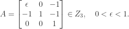
for an
We have
![\notag A^{-1} = \begin{bmatrix} \displaystyle\frac{1}{\epsilon}& 0& \displaystyle\frac{1}{\epsilon}\\[\bigskipamount] \displaystyle\frac{1}{\epsilon}& 1 & \displaystyle\frac{1 + \epsilon}{\epsilon}\\[\bigskipamount] 0& 0& 1 \end{bmatrix} \ge 0,](https://s0.wp.com/latex.php?latex=%5Cnotag++A%5E%7B-1%7D+%3D++++%5Cbegin%7Bbmatrix%7D++++++++%5Cdisplaystyle%5Cfrac%7B1%7D%7B%5Cepsilon%7D%26+0%26+%5Cdisplaystyle%5Cfrac%7B1%7D%7B%5Cepsilon%7D%5C%5C%5B%5Cbigskipamount%5D++++++++%5Cdisplaystyle%5Cfrac%7B1%7D%7B%5Cepsilon%7D%26+1+%26+%5Cdisplaystyle%5Cfrac%7B1+%2B+%5Cepsilon%7D%7B%5Cepsilon%7D%5C%5C%5B%5Cbigskipamount%5D++++++++++++++++++0%26+++++++++++0%26+++++1++++%5Cend%7Bbmatrix%7D+%5Cge+0%2C+&bg=ffffff&fg=222222&s=0&c=20201002)
so 


and this lower bound can be arbitrarily large. One can verify experimentally that numerical instability is possible when 
Stationery Iterative Methods
A stationery iterative method for solving a linear system 


Matrix Square Root
The principal square root 
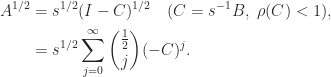
This expression does not necessarily provide the best way to compute
Singular M-Matrices
The theory of 


H-Matrices
A more general concept is that of 


References
This is a minimal set of references, which contain further useful references within.
- Abraham Berman and Robert J. Plemmons, Nonnegative Matrices in the Mathematical Sciences, Society for Industrial and Applied Mathematics, Philadelphia, PA, USA, 1994.
- R. E. Funderlic and M. Neumann and R. J. Plemmons
Decompositions of Generalized Diagonally Dominant Matrices, Numer. Math. 40, 57–69, 1982.
- Nicholas J. Higham, Accuracy and Stability of Numerical Algorithms, second edition, Society for Industrial and Applied Mathematics, Philadelphia, PA, USA, 2002. (Chapter 8.)
- Nicholas J. Higham, Functions of Matrices: Theory and Computation, Society for Industrial and Applied Mathematics, Philadelphia, PA, USA, 2008. (Section 6.8.3.)
Related Blog Posts
- What Is a Matrix Square Root? (2020)
- What Is a Symmetric Positive Definite Matrix? (2020)
- What is Numerical Stability? (2020)
This article is part of the “What Is” series, available from https://nhigham.com/category/what-is and in PDF form from the GitHub repository https://github.com/higham/what-is.

Excuse me, can you prove the inequalities for the inveres M-matrix bound, i.e |A^{-1}| \leq M(A)^{-1} ? Thanks in advance
For an M-matrix, M(A) = A so that bound is trivial. The bound always holds for triangular A, as noted above, but does not always hold in general.
Thankyou for the replies, Sir. First of all, i have already read an article about M-Matrices and H-Matrices (https://www.sciencedirect.com/science/article/abs/pii/S0024379519305087). In that article (pg 5), there is a statement :
A well known relationship between an invertible H-matrix and its comparison matrix due to Ostrowski [10] states that, for an invertible H-matrix A ∈ C^{n×n}, the inequality |A^{−1}| ≤ (M(A))^{−1} holds.
I am confused to prove this statement. Any advice?
Please is there any result that shows that the inverse of a strictly diagonally dominant matrix is also strictly diagonally dominant?
I checked this numerically which holds, but could not find any analytic proof to support this.
Many thanks
It’s not true: A = full(gallery(‘tridiag’,5,1,2.5,1)) is a counterexample.
However, see Theorem 6 in https://nhigham.com/2021/04/08/what-is-a-diagonally-dominant-matrix/ for a partial result along these lines.