An 


The definition says that the inner product of the 


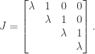
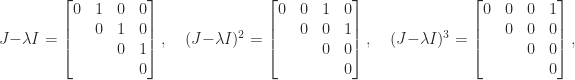
For a general diagonalizable matrix, 


Many equivalent conditions to
The normal matrices include the classes of matrix given in this table:
| Real | Complex |
|---|---|
| Diagonal | Diagonal |
| Symmetric | Hermitian |
| Skew-symmetric | Skew-Hermitian |
| Orthogonal | Unitary |
| Circulant | Circulant |
Circulant matrices are
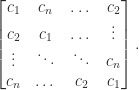
They are diagonalized by a unitary matrix known as the discrete Fourier transform matrix, which has 

A normal matrix is not necessarily of the form given in the table, even for 

![\notag \left[\begin{array}{@{\mskip2mu}rr@{\mskip2mu}} a & b\\ b & c \end{array}\right], \quad \left[\begin{array}{@{}rr@{\mskip2mu}} a & b\\ -b & a \end{array}\right].](https://s0.wp.com/latex.php?latex=%5Cnotag++++%5Cleft%5B%5Cbegin%7Barray%7D%7B%40%7B%5Cmskip2mu%7Drr%40%7B%5Cmskip2mu%7D%7D++++++a+%26+b%5C%5C++++++b+%26+c++++%5Cend%7Barray%7D%5Cright%5D%2C+%5Cquad++++%5Cleft%5B%5Cbegin%7Barray%7D%7B%40%7B%7Drr%40%7B%5Cmskip2mu%7D%7D++++++a+%26+b%5C%5C+++++-b+%26+a++++%5Cend%7Barray%7D%5Cright%5D.+&bg=ffffff&fg=222222&s=0&c=20201002)
The first matrix is symmetric. The second matrix is of the form 
![J = \bigl[\begin{smallmatrix}\!\phantom{-}0 & 1\\\!-1 & 0 \end{smallmatrix}\bigr]](https://s0.wp.com/latex.php?latex=J+%3D+%5Cbigl%5B%5Cbegin%7Bsmallmatrix%7D%5C%21%5Cphantom%7B-%7D0+%26+1%5C%5C%5C%21-1+%26+0+%5Cend%7Bsmallmatrix%7D%5Cbigr%5D&bg=ffffff&fg=222222&s=0&c=20201002)


It is natural to ask what the commutator 

In the polar decomposition 


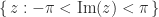
The field of values, also known as the numerical range, is defined for 
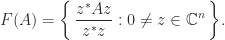
The set 
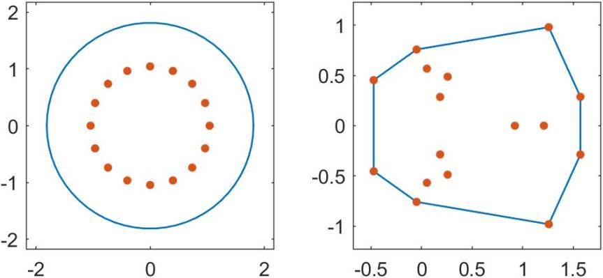
gallery('smoke',16) and that on the right is for the circulant matrix gallery('circul',x) with x constructed as x = randn(16,1); x = x/norm(x).
Measures of Nonnormality
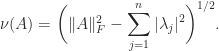
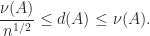
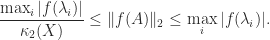
How can we measure the degree of nonnormality of a matrix? Let 


Henrici (1962) derived an upper bound for 
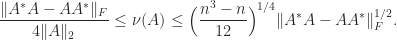
The distance to normality is

This quantity can be computed by an algorithm of Ruhe (1987). It is trivially bounded above by
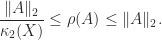
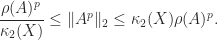
Normal matrices are a particular class of diagonalizable matrices. For diagonalizable matrices various bounds are available that depend on the condition number of a diagonalizing transformation. Since such a transformation is not unique, we take a diagonalization

Here are some examples of such bounds. We denote by 
- By taking norms in the eigenvalue-eigenvector equation
we obtain
. Taking norms in
. Hence
- If
and its eigenvalues are ordered
, then (Ruhe, 1975)
Note that for
the previous upper bound is sharper.
- For any real
,
- For any function
defined on the spectrum of

For normal 
References
This is a minimal set of references, which contain further useful references within.
- L. Elsner and Kh.D. Ikramov, Normal Matrices: An Update, Linear Algebra Appl 285, 291–303, 1998.
- L. Elsner and M. H. C. Paardekooper, On Measures of Nonnormality of Matrices, Linear Algebra Appl. 92, 107–124, 1987.
- Robert Grone, Charles Johnson, Eduardo Sa, and Henry Wolkowicz, Normal Matrices, Linear Algebra Appl. 87, 213–225, 1987
- Peter Henrici, Bounds for Iterates, Inverses, Spectral Variation and Fields of Values of Non-Normal Matrices, Numer. Math. 4, 24–40, 1962.
- Lajos László, An Attainable Lower Bound for the Best Normal Approximation, SIAM J. Matrix Anal. Appl. 15 (3), 1035–1043, 1994.
- Axel Ruhe, On the Closeness of Eigenvalues and Singular Values Of Almost Normal Matrices, Linear Algebra Appl. 11, 87–94, 1975.
- Axel Ruhe, Closest Normal Matrix Finally Found!, BIT 27, 585–598, 1987.
 , where
  is the matrix exponential. Just as in the scalar case, the matrix logarithm is not unique, since if
  for any integer
  . However, for matrices the nonuniqueness is complicated by the presence of repeated eigenvalues. For example, the matrix
 identity matrix
  for any
  , whereas the obvious logarithms are the diagonal matrices
  , for integers
  ,
,  , and
, and  . Notice that the repeated eigenvalue
  ,
,  , and
, and  in
in  . This is characteristic of nonprimary logarithms, and in some applications such strange logarithms may be required—an example is the embeddability problem for Markov chains.
 but not for odd
  ,
,![\notag X = \pi\left[\begin{array}{@{}rr@{}} 0 & 1\\ -1 & 0 \end{array}\right]](https://s0.wp.com/latex.php?latex=%5Cnotag++++X+%3D++%5Cpi%5Cleft%5B%5Cbegin%7Barray%7D%7B%40%7B%7Drr%40%7B%7D%7D++++++++++++++0+%26+1%5C%5C++++++++++++++-1+%26+0+++++++++++++%5Cend%7Barray%7D%5Cright%5D+&bg=ffffff&fg=222222&s=0&c=20201002)
 , as does
  for any nonsingular
  , since
  .
. . From this point on we assume that
 ![\notag \begin{aligned} \log A &= \int_0^1 (A-I)\bigl[ t(A-I) + I \bigr]^{-1} \,\mathrm{d}t, \\ \log(I+X) &= X - \frac{X^2}{2} + \frac{X^3}{3} - \frac{X^4}{4} + \cdots, \quad \rho(X)<1, \end{aligned}](https://s0.wp.com/latex.php?latex=%5Cnotag+%5Cbegin%7Baligned%7D+++++++%5Clog+A++%26%3D+%5Cint_0%5E1+%28A-I%29%5Cbigl%5B+t%28A-I%29+%2B+I+%5Cbigr%5D%5E%7B-1%7D+%5C%2C%5Cmathrm%7Bd%7Dt%2C+%5C%5C+++++%5Clog%28I%2BX%29+%26%3D+X+-+%5Cfrac%7BX%5E2%7D%7B2%7D+%2B+%5Cfrac%7BX%5E3%7D%7B3%7D++++++++++++++++++++-+%5Cfrac%7BX%5E4%7D%7B4%7D+%2B+%5Ccdots%2C+%5Cquad+%5Crho%28X%29%3C1%2C+%5Cend%7Baligned%7D+&bg=ffffff&fg=222222&s=0&c=20201002)
 . A useful relation is
 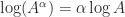 for
for ![\alpha\in[-1,1]](https://s0.wp.com/latex.php?latex=%5Calpha%5Cin%5B-1%2C1%5D&bg=ffffff&fg=222222&s=0&c=20201002) , with important special cases
, with important special cases  and
and 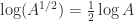 (where the square root is the principal square root). Recurring the latter expression gives, for any positive integer
 is small enough that
  can be efficiently approximated by Padé approximation. The MATLAB function
  with
with  is a factorization
  with
with  orthonormal and
  upper trapezoidal. The
  factor has the form
 ![R = \left[\begin{smallmatrix}R_1\\ 0\end{smallmatrix}\right]](https://s0.wp.com/latex.php?latex=R+%3D+%5Cleft%5B%5Cbegin%7Bsmallmatrix%7DR_1%5C%5C+0%5Cend%7Bsmallmatrix%7D%5Cright%5D&bg=ffffff&fg=222222&s=0&c=20201002) , where
, where  is
is ![\notag A = QR = \begin{array}[b]{@{\mskip-20mu}c@{\mskip0mu}c@{\mskip-1mu}c@{}} & \mskip10mu\scriptstyle n & \scriptstyle m-n \\ \mskip15mu \begin{array}{r} \scriptstyle m \end{array}~ & \multicolumn{2}{c}{\mskip-15mu \left[\begin{array}{c@{~}c@{~}} Q_1 & Q_2 \end{array}\right] } \end{array} \mskip-10mu \begin{array}[b]{@{\mskip-25mu}c@{\mskip-20mu}c@{}} \scriptstyle n \\ \multicolumn{1}{c}{ \left[\begin{array}{@{}c@{}} R_1\\ 0 \end{array}\right]} & \mskip-12mu\ \begin{array}{l} \scriptstyle n \\ \scriptstyle m-n \end{array} \end{array} = Q_1 R_1.](https://s0.wp.com/latex.php?latex=%5Cnotag++++A+%3D+QR+++++%3D++++%5Cbegin%7Barray%7D%5Bb%5D%7B%40%7B%5Cmskip-20mu%7Dc%40%7B%5Cmskip0mu%7Dc%40%7B%5Cmskip-1mu%7Dc%40%7B%7D%7D++++%26+%5Cmskip10mu%5Cscriptstyle+n+%26+%5Cscriptstyle+m-n++%5C%5C+++++++%5Cmskip15mu++++++++++%5Cbegin%7Barray%7D%7Br%7D++++++++++++++%5Cscriptstyle+m++++++++++%5Cend%7Barray%7D%7E++++%26+++++++%5Cmulticolumn%7B2%7D%7Bc%7D%7B%5Cmskip-15mu++++++++++%5Cleft%5B%5Cbegin%7Barray%7D%7Bc%40%7B%7E%7Dc%40%7B%7E%7D%7D++++++++++++++++++Q_1+%26+Q_2++++++++++++++++%5Cend%7Barray%7D%5Cright%5D+++++++%7D++++%5Cend%7Barray%7D+%5Cmskip-10mu++++%5Cbegin%7Barray%7D%5Bb%5D%7B%40%7B%5Cmskip-25mu%7Dc%40%7B%5Cmskip-20mu%7Dc%40%7B%7D%7D++++%5Cscriptstyle+n++++%5C%5C++++%5Cmulticolumn%7B1%7D%7Bc%7D%7B++++++++%5Cleft%5B%5Cbegin%7Barray%7D%7B%40%7B%7Dc%40%7B%7D%7D++++++++++++++++++R_1%5C%5C++++++++++++++++++0++++++++++++++%5Cend%7Barray%7D%5Cright%5D%7D++++%26+%5Cmskip-12mu%5C++++++++++%5Cbegin%7Barray%7D%7Bl%7D++++++++++++++%5Cscriptstyle+n+%5C%5C++++++++++++++%5Cscriptstyle+m-n++++++++++%5Cend%7Barray%7D++++%5Cend%7Barray%7D++++%3D+Q_1+R_1.+&bg=ffffff&fg=222222&s=0&c=20201002)
 is the reduced (also called economy-sized, or thin) QR factorization.
 is symmetric positive definite. Since
  , we can take
  . The resulting
  has orthonormal columns because
 and obtain another QR factorization.)
 implies
  while
while  implies
  , so
, so  . Furthermore,
  gives
gives  , so the columns of
  span the null space of
  .
. is not guaranteed to be orthonormal to the working precision. The modified Gram–Schmidt method (a variation of the classical method) is better behaved numerically in that
  for some constant
  , where
  is the unit roundoff, so the loss of orthogonality is bounded.
 as a product of orthogonal matrices that are chosen to reduce
 ![\notag \qquad\qquad\qquad\qquad A^{(k)} = Q_{k-1}^T A = \begin{array}[b]{@{\mskip35mu}c@{\mskip20mu}c@{\mskip-5mu}c@{}c} \scriptstyle k-1 & \scriptstyle 1 & \scriptstyle n-k & \\ \multicolumn{3}{c}{ \left[\begin{array}{c@{\mskip10mu}cc} R_{k-1} & y_k & B_k \\ 0 & z_k & C_k \end{array}\right]} & \mskip-12mu \begin{array}{c} \scriptstyle k-1 \\ \scriptstyle m-k+1 \end{array} \end{array}, \qquad\qquad\qquad\qquad (*)](https://s0.wp.com/latex.php?latex=%5Cnotag+++%5Cqquad%5Cqquad%5Cqquad%5Cqquad++++A%5E%7B%28k%29%7D+%3D+Q_%7Bk-1%7D%5ET+A+%3D++++%5Cbegin%7Barray%7D%5Bb%5D%7B%40%7B%5Cmskip35mu%7Dc%40%7B%5Cmskip20mu%7Dc%40%7B%5Cmskip-5mu%7Dc%40%7B%7Dc%7D++++%5Cscriptstyle+k-1+%26++++%5Cscriptstyle+1+%26++++%5Cscriptstyle+n-k+%26++++%5C%5C++++%5Cmulticolumn%7B3%7D%7Bc%7D%7B++++%5Cleft%5B%5Cbegin%7Barray%7D%7Bc%40%7B%5Cmskip10mu%7Dcc%7D++++R_%7Bk-1%7D+%26+y_k++%26+B_k+%5C%5C++++++++0+++%26+z_k++%26+C_k++++%5Cend%7Barray%7D%5Cright%5D%7D++++%26+%5Cmskip-12mu++++%5Cbegin%7Barray%7D%7Bc%7D++++%5Cscriptstyle+k-1+%5C%5C++++%5Cscriptstyle+m-k%2B1++++%5Cend%7Barray%7D++++%5Cend%7Barray%7D%2C+++%5Cqquad%5Cqquad%5Cqquad%5Cqquad+%28%2A%29+&bg=ffffff&fg=222222&s=0&c=20201002)
 is upper triangular and
  is a product of Householder transformations or Givens rotations. Working on
 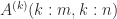 we now apply a Householder transformation or
  Givens rotations in order to zero out the last
  and thereby take the matrix one step closer to upper trapezoidal form.
 , for some constant
  .
. satisfies
 .
. . In its basic form, this method is not recommended unless
  , the column of largest
  , the
, the  then the
  th columns of
  are interchanged. The result is a factorization
  , where
  is a permutation matrix and


 nonsingular, and the rank of
 and
and  ,
,  is of order
  times larger than the smallest singular value for small
  and
and  is invariant under QR factorization with column pivoting.
 .
. is rank-revealing. Computing such a permutation is impractical, but heuristic algorithms for producing an approximate rank-revealing factorization are available.
 where
where  is the characteristic polynomial. This statement is not simply the substitution “
 ”, which is not valid since
  term. Rather, for an

 Jordan block with eigenvalue
  :
:
 . In general, for an
  Jordan block
  with eigenvalue
  is zero apart from a
  , and
, and  .
. , where
 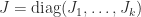 and each
  is an
is an  Jordan block with eigenvalue
  . The characteristic polynomial of
  . Note that
  for all
  for any polynomial
  . Then
 is zero because it contains a factor
  and this factor is zero, as noted above. Hence
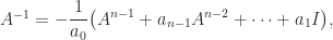
  and therefore
  of an
of an  is the transposed matrix of cofactors, where a cofactor is a signed sum of products of
  entries of
  . With
  , each entry of
  can be written
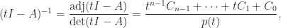
 ,
,  ,
,  not depending on
 , …,
, …,  gives
gives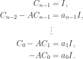
 , the second by
  , and so on, and adding, gives
 is expressible as a linear combination of
  ,
, 
 .
. for any
  can be expressed as a linear combination of
  can be written
  for some scalars
  , …,
, …,  . However, the
  depend on
  :
:
 .
. then applying the theorem to
  , or
, or

 and taking the trace in
  , leading to
 of the characteristic polynomial are typically numerically unstable.
 for all nonnegative
  , for all nonnegative
  , adding “I have not thought it necessary to undertake the labour of a formal proof of the theorem in the general case of a matrix of any degree.” Hamilton had proved the result for quaternions in 1853. Cayley actually discovered a more general version of the Cayley–Hamilton theorem, which appears in an 1857 letter to Sylvester but not in any of his published work: if the square matrices
  then
then  .
.