What Is the Kac–Murdock–Szegö Matrix?

The Kac–Murdock–Szegö matrix is the symmetric Toeplitz matrix

\notag A_n(\rho) = \begin{bmatrix}    1          & \rho       & \rho^2 & \dots  & \rho^{n-1} \\    \rho       & 1          & \rho   & \dots  & \rho^{n-2} \\    \rho^2     & \rho       & 1      & \ddots & \vdots     \\    \vdots     & \vdots     & \ddots & \ddots & \rho       \\    \rho^{n-1} & \rho^{n-2} & \dots  & \rho   & 1 \end{bmatrix} \in\mathbb{R}^{n\times n}. \qquad(1)

It was considered by Kac, Murdock, and Szegö (1953), who investigated its spectral properties. It arises in the autoregressive AR(1) model in statistics and signal processing.

The matrix is singular for \rho=1, as A_n(1) is the rank-1 matrix ee^T, and it is also rank-1 for \rho = -1, as in this case every column is a multiple of the vector with alternating elements \pm 1. The determinant \det(A_n(\rho)) = (1-\rho^2)^{n-1}. For \rho \ne \pm 1, A_n is nonsingular and the inverse is the tridiagonal (but not Toeplitz) matrix

\notag   A_n(\rho)^{-1} = \displaystyle\frac{1}{1-\rho^2}   \begin{bmatrix}    1      & -\rho    & 0        & \dots  & \dots    & 0      \\    -\rho  & 1+\rho^2 & -\rho    & \dots  & \dots    & 0      \\    0      & -\rho    & 1+\rho^2 & \ddots & \dots    & \vdots \\    \vdots & \vdots   & \ddots   & \ddots & \ddots   & 0      \\    0      & \dots    & \dots    & -\rho  & 1+\rho^2 & -\rho  \\    0      & \dots    & \dots    & 0      & -\rho    & 1   \end{bmatrix}. \qquad (2)

For -1 < \rho < 1, A_n(\rho) is positive definite, since every leading principal submatrix has positive determinant, as can also be seen by noting that the inverse is diagonally dominant with positive diagonal, so that A_n^{-1} is positive definite and hence A_n is positive definite.

For -1 \le \rho \le 1, A_n(\rho) is positive semidefinite, so it is a correlation matrix for \rho in this range.

For 0 \le \rho \le 1, A_n(\rho) is totally nonnegative, that is. every submatrix has nonnegative determinant. For 0 < \rho < 1, we know that A_n(\rho) is nonsingular, and it is clearly irreducible, and together with the total nonnegativity these properties imply that the eigenvalues are distinct and positive (this can also be deduced from the fact that the inverse is tridiagonal with nonzero subdiagonal and superdiagonal entries).

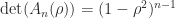
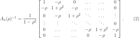
It is straightforward to verify that A_n has a factorization A_n = LDL^* with L the inverse of a unit lower bidiagonal matrix:

\notag  L =   \begin{bmatrix}    1     &          &          &        &\\    -\rho & 1        &          &        &\\          & -\rho    & 1        &        &\\          &          & \ddots   & \ddots &\\          &          &          &-\rho   &1   \end{bmatrix}^{-1}, \quad  D = \mathrm{diag}(1, 1-\rho^2, 1-\rho^2, \dots, 1-\rho^2).  \qquad (3)

This factorization can be used to prove all the properties stated above.

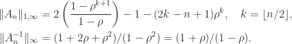
From (1) and (2) we can derive the formulas

\notag    \begin{aligned}   \|A_n\|_{1,\infty} &=        2 \left(\displaystyle\frac{1-\rho^{k+1}}{1-\rho}\right)        -1 - (2k-n+1) \rho^k,    \quad k = \lfloor n/2 \rfloor, \\   \|A_n^{-1}\|_{\infty} &= (1+2\rho+\rho^2)/(1-\rho^2) = (1+\rho)/(1-\rho).    \end{aligned}

Hence we have an explicit formula for the condition number
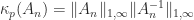
 \kappa_p(A_n) = \|A_n\|_{1,\infty} \|A_n^{-1}\|_{1,\infty} for p = 1,\infty.

We can allow \rho to be complex, in which case the definition (1) is modified to conjugate the elements below the diagonal. The factorization A = LDL^* continues to hold with D in (2) replaced by \mathrm{diag}(1, 1-|\rho|^2, 1-|\rho|^2, \dots, 1-|\rho|^2).

The Kac–Murdock–Szegö matrix (for real or complex \rho) can be generated in MATLAB as gallery('kms',n,rho).

References

This is a minimal set of references, which contain further useful references within.

Related Blog Posts

This article is part of the “What Is” series, available from https://nhigham.com/category/what-is and in PDF form from the GitHub repository https://github.com/higham/what-is.

Leave a comment