
The two-part minisymposium Bohemian Matrices and Applications, organized by Rob Corless and I, took place at the SIAM Annual Meeting, July 22 and 23, 2021. This page makes available slides from some of the talks.
The minisymposium followed a two-part minisymposium on Bohemian matrices at the 2019 ICIAM meeting in Valencia and a 3-day workshop on Bohemian matrices in Manchester in 2018.
For more on Bohemian matrices see the Bohemian matrices website.
Minisymposium description: Bohemian matrices are matrices with entries drawn from a fixed discrete set of small integers (or some other discrete set). The term is a contraction of BOunded HEight Matrix of Integers. Such matrices arise in many applications, and include 

Putting Skew-Symmetric Tridiagonal Bohemians on the Calendar. Robert M. Corless, Western University, Canada. Abstract. Rob did not use slides but gave his talk using this paper and this Maple worksheet.
Determinants of Normalized Bohemian Upper Hessenberg Matrices. Massimiliano Fasi, Örebro University, Sweden; Jishe Feng, Longdong University, China; Gian Maria Negri Porzio, University of Manchester, United Kingdom. Abstract. Slides.
Experiments on Upper Hessenberg and Toeplitz Bohemians. Eunice Chan, Western University, Canada. Abstract. Slides.
Eigenvalues of Magic Squares and Related Bohemian Matrices. Hariprasad Manjunath Hegde, Indian Institute of Science, Bengaluru, India. Abstract. Slides.
Calculating the 3D Kings Multiplicity Constant. Nicholas Cohen and Neil Calkin, Clemson University, U.S. Abstract. Slides.
Bohemian Inners Inverses: A First Step Toward Bohemian Generalized Inverses. Laureano Gonzalez-Vega, Universidad de Cantabria, Spain; Juan Rafael Sendra, Universidad Alcalá de Henares, Spain; Juana Sendra Pons, Universidad Politécnica de Madrid, Spain. Abstract. Slides.
Recent Progress in the Rational Factorisation of Integer Matrices. Matthew Lettington, Cardiff University, United Kingdom. Abstract. Slides.
Which Columns are Independent? Why does Row Rank = Column Rank? Gilbert Strang, Massachusetts Institute of Technology, U.S. Abstract. Slides.
Bohemian Matrices: the Symbolic Computation Approach. Juana Sendra, Universidad Autónoma de Madrid, Spain; Laureano González-Vega, Universidad de Estudios Financieros en Madrid, Spain; Juan Rafael Sendra, Universidad Alcalá de Henares, Spain. Abstract. Slides.
 is totally positive if every minor is positive. It is totally nonnegative if every minor is nonnegative. These definitions require, in particular, that all the matrix elements must be nonnegative or positive, as must
  .
. are totally nonnegative then so is
  .
.![\alpha = [\alpha_1,\alpha_2,\dots,\alpha_k]](https://s0.wp.com/latex.php?latex=%5Calpha+%3D+%5B%5Calpha_1%2C%5Calpha_2%2C%5Cdots%2C%5Calpha_k%5D&bg=ffffff&fg=222222&s=0&c=20201002) is an index vector of order
is an index vector of order  if its components are integers from the set
  satisfying
  . If
. If  and
and  are index vectors of order
  , respectively, then
  denotes the
  matrix with (
 ) element
  .
. ,
,  , and
, and  . If
. If  then
then
 of order
  , (1) reduces to the well-known relation
  , while when
  , (1) reduces to the definition of matrix multiplication.
 comprises the indices not in
  :
:
 , with
  . The Hilbert matrix is a particular case of a Cauchy matrix
  , with
  for given vectors
  . A Cauchy matrix is totally positive if
  and
and  , which follows from the formula

 satisfy
 is defined by
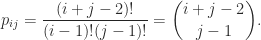
 (see the section below on bidiagonal factorizations).
 with off-diagonal elements given by
  with
with  , illustrated by
![A([1,2],[2,3]) = \bigl[\begin{smallmatrix} \theta & \theta \\ 1 & \theta \end{smallmatrix}\bigr]](https://s0.wp.com/latex.php?latex=A%28%5B1%2C2%5D%2C%5B2%2C3%5D%29+%3D++++%5Cbigl%5B%5Cbegin%7Bsmallmatrix%7D++++%5Ctheta+%26+%5Ctheta+%5C%5C++++1++++++%26+%5Ctheta++++%5Cend%7Bsmallmatrix%7D%5Cbigr%5D+&bg=ffffff&fg=222222&s=0&c=20201002) has nonpositive determinant. However, the
has nonpositive determinant. However, the  , with
 with all elements
  on and below the superdiagonal, illustrated for
  by
by
 zero eigenvalues, which appear in a single Jordan block, and its largest eigenvalue is
  . In MATLAB, this matrix can be generated by
  bidiagonal matrix factorized into a product of elementary nonnegative bidiagonal matrices (nonnegative means that the elements of the matrix are nonnegative):
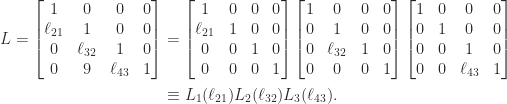
 ,
,  , and
, and  are totally nonnegative, so
  is totally nonnegative by Theorem 1. With
  , we have
 nonnegative bidiagonal matrix is totally nonnegative.
 , where
 denotes the submatrix of
  and column
  . If
. If  has a checkerboard (alternating) sign pattern. Indeed, we can write
  , where
  and
and  has nonnegative elements, and in fact it can be shown that
  is irreducible if there does not exist a permutation matrix
  such that
 and
and  are square, nonempty submatrices.
 . It is known that the eigenvector
  associated with
  has
has  sign changes, that is,
  and (
and ( have opposite signs for
  (any zero elements are deleted before counting sign changes). Note that for
  , we already know from Perron–Frobenius theory that there is a positive eigenvector
  . This result is illustrated by the Pascal matrix above:
 is totally positive for some positive integer
 totally nonnegative and the
  .
. for
for  , which guarantees the existence of an LU factorization. That the elements of
  and computes
  , since
  . Thus
  ,
,  . For
. For  ,
,  ; for
; for  ,
,  . Thus
  for all
  and hence
  . But
. But  , so
, so  .
. the computed factors
  and
and  will have nonnegative elements and so from the standard backward error result for LU factorization,

 and hence

 is a diagonal matrix with positive diagonal entries and
  and
and  are unit lower and unit upper bidiagonal matrices, respectively, with the first
  entries along the subdiagonal of
  zero and the rest nonnegative.
 subdiagonal entries of
  principal minors (ones based on submatrices centred on the diagonal) and
  minors in total. However, it is not necessary to check all these minors to test for total positivity.
 for all index vectors
 ![[1,2,\dots,k]](https://s0.wp.com/latex.php?latex=%5B1%2C2%2C%5Cdots%2Ck%5D&bg=ffffff&fg=222222&s=0&c=20201002) and the entries of the other are
and the entries of the other are  minors need to be tested. Gasca and Peña have also show that total nonnegativity can be tested by checking about
  minors. A more efficient way to test for total nonnegativity is to compute the factorization in Theorem 6 and check the signs of the entries.
 the spectral radius of
  such that
  .
. ,
, ,
, for any eigenvalue
  with
with  .
. , is called the Perron vector.
 matrices. Here are some interesting cases.
![A = \bigl[\begin{smallmatrix}0 & 1 \\ 0 & 0 \end{smallmatrix}\bigr]](https://s0.wp.com/latex.php?latex=A+%3D+%5Cbigl%5B%5Cbegin%7Bsmallmatrix%7D0+%26+1+%5C%5C+0+%26+0+%5Cend%7Bsmallmatrix%7D%5Cbigr%5D&bg=ffffff&fg=222222&s=0&c=20201002) : Theorem 1 says that
: Theorem 1 says that  is an eigenvalue and and that it has a nonnegative eigenvector. Indeed
 ![[1~0]^T](https://s0.wp.com/latex.php?latex=%5B1%7E0%5D%5ET&bg=ffffff&fg=222222&s=0&c=20201002) is an eigenvector. Note that
is an eigenvector. Note that  is a repeated eigenvalue.
![A = \bigl[\begin{smallmatrix}0 & 1 \\ 1 & 0 \end{smallmatrix}\bigr]](https://s0.wp.com/latex.php?latex=A+%3D+%5Cbigl%5B%5Cbegin%7Bsmallmatrix%7D0+%26+1+%5C%5C+1+%26+0+%5Cend%7Bsmallmatrix%7D%5Cbigr%5D&bg=ffffff&fg=222222&s=0&c=20201002) :
:  and
and ![[1~1]^T/2](https://s0.wp.com/latex.php?latex=%5B1%7E1%5D%5ET%2F2&bg=ffffff&fg=222222&s=0&c=20201002) is the Perron vector for the Perron root
is the Perron vector for the Perron root ![A = \bigl[\begin{smallmatrix}1 & 1 \\ 1 & 1 \end{smallmatrix}\bigr]](https://s0.wp.com/latex.php?latex=A+%3D+%5Cbigl%5B%5Cbegin%7Bsmallmatrix%7D1+%26+1+%5C%5C+1+%26+1+%5Cend%7Bsmallmatrix%7D%5Cbigr%5D&bg=ffffff&fg=222222&s=0&c=20201002) : Theorem 3 says that
: Theorem 3 says that  is an eigenvalue with positive eigenvector and that the other eigenvalue has modulus less than
  . Indeed the eigenvalues are the Perron root
 is an eigenvalue of
 ![[1~1~1]^T/3](https://s0.wp.com/latex.php?latex=%5B1%7E1%7E1%5D%5ET%2F3&bg=ffffff&fg=222222&s=0&c=20201002) . Two of the eigenvalues are complex, however, and all three eigenvalues have modulus 1, as they must because
. Two of the eigenvalues are complex, however, and all three eigenvalues have modulus 1, as they must because  , where
 ![e = [1,1,\dots,1]^T](https://s0.wp.com/latex.php?latex=e+%3D+%5B1%2C1%2C%5Cdots%2C1%5D%5ET&bg=ffffff&fg=222222&s=0&c=20201002) , which means that
, which means that  . Since
  for any norm, by taking the
  -norm we conclude that
  is the Perron vector of
  then
then
 (since
  ).
). . If
. If  and Theorem 4 says that
  . We illustrate this result in MATLAB using a scaled magic square matrix.
 , as
, as  is the rank-
 , and it is also rank-
 , as in this case every column is a multiple of the vector with alternating elements
 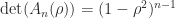 . For
. For  ,
,  is nonsingular and the inverse is the tridiagonal (but not Toeplitz) matrix
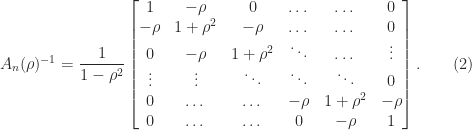
 ,
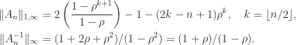
,  is positive definite, since every leading principal submatrix has positive determinant, as can also be seen by noting that the inverse is diagonally dominant with positive diagonal, so that
  is positive definite and hence
  ,
,  in this range.
 ,
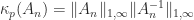
,  , we know that
  with
with 
 for
for  .
. continues to hold with
  replaced by
  .
.