What is the Polar Decomposition?

A polar decomposition of $A\in\mathbb{C}^{m \times n}$ with $m \ge n$ is a factorization $A = UH$ , where $U\in\mathbb{C}^{m \times n}$ has orthonormal columns and $H\in\mathbb{C}^{n \times n}$ is Hermitian positive semidefinite. This decomposition is a generalization of the polar representation $z = r \mathrm{e}^{\mathrm{i}\theta}$ of a complex number, where $H$ corresponds to $r\ge 0$ and $U$ to $\mathrm{e}^{\mathrm{i}\theta}$ . When $A$ is real, $H$ is symmetric positive semidefinite. When $m = n$ , $U$ is a square unitary matrix (orthogonal for real $A$ ).

We have $A^*A = H^*U^*UH = H^2$ , so $H = (A^*\!A)^{1/2}$ , which is the unique positive semidefinite square root of $A^*A$ . When $A$ has full rank, $H$ is nonsingular and $U = AH^{-1}$ is unique, and in this case $U$ can be expressed as

$U = \displaystyle\frac{2}{\pi} A \displaystyle\int_{0}^{\infty} (t^2I+A^*\!A)^{-1}\, \mathrm{d}t.$

An example of a polar decomposition is

$A = \left[\begin{array}{@{}rr} 4 & 0\\ -5 & -3\\ 2 & 6 \end{array}\right] = \sqrt{2}\left[\begin{array}{@{}rr} \frac{1}{2} & -\frac{1}{6}\\[\smallskipamount] -\frac{1}{2} & -\frac{1}{6}\\[\smallskipamount] 0 & \frac{2}{3} \end{array}\right] \cdot \sqrt{2}\left[\begin{array}{@{\,}rr@{}} \frac{9}{2} & \frac{3}{2}\\[\smallskipamount] \frac{3}{2} & \frac{9}{2} \end{array}\right] \equiv UH.$

For an example with a rank-deficient matrix consider

$A = \begin{bmatrix} 0 & 1 & 0 \\ 0 & 0 & 1 \\ 0 & 0 & 0 \end{bmatrix},$

for which $A^*A = \mathrm{diag}(0,1,1)$ and so $H = \mathrm{diag}(0,1,1)$ . The equation $A = UH$ then implies that

$U = \begin{bmatrix} 0 & 1 & 0 \\ 0 & 0 & 1 \\ \theta & 0 & 0 \end{bmatrix}, \quad |\theta| = 1,$

so $U$ is not unique.

The polar factor $U$ has the important property that it is a closest matrix with orthonormal columns to $A$ in any unitarily invariant norm. Hence the polar decomposition provides an optimal way to orthogonalize a matrix. This method of orthogonalization is used in various applications, including in quantum chemistry, where it is called Löwdin orthogonalization. Most often, though, orthogonalization is done through QR factorization, trading optimality for a faster computation.

An important application of the polar decomposition is to the orthogonal Procrustes problem¹

$\min \bigl\{\, \|A-BW\|_F: W \in \mathbb{C}^{n\times n},\; W^*W = I \,\bigr\},$

where $A,B\in\mathbb{C}^{m\times n}$ and the norm is the Frobenius norm $\|A\|_F^2 = \sum_{i,j} |a_{ij}|^2$ . This problem, which arises in factor analysis and in multidimensional scaling, asks how closely a unitary transformation of $B$ can reproduce $A$ . Any solution is a unitary polar factor of $B^*\!A$ , and there is a unique solution if $B^*\!A$ is nonsingular. Another application of the polar decomposition is in 3D graphics transformations. Here, the matrices are $3\times 3$ and the polar decomposition can be computed by exploiting a relationship with quaternions.

For a square nonsingular matrix $A$ , the unitary polar factor $U$ can be computed by a Newton iteration:

$X_{k+1} = \displaystyle\frac{1}{2} (X_k + X_k^{-*}), \quad X_0 = A.$

The iterates $X_k$ converge quadratically to $U$ . This is just one of many iterations for computing $U$ and much work has been done on the efficient implementation of these iterations.

If $A = P \Sigma Q^*$ is a singular value decomposition (SVD), where $P\in\mathbb{C}^{m\times n}$ has orthonormal columns, $Q\in\mathbb{C}^{n\times n}$ is unitary, and $\Sigma$ is square and diagonal with nonnegative diagonal elements, then

$A = PQ^* \cdot Q \Sigma Q^* \equiv UH,$

where $U$ has orthonormal columns and $H$ is Hermitian positive semidefinite. So a polar decomposition can be constructed from an SVD. The converse is true: if $A = UH$ is a polar decomposition and $H = Q\Sigma Q^*$ is a spectral decomposition ( $Q$ unitary, $D$ diagonal) then $A = (UQ)\Sigma Q^* \equiv P \Sigma Q^*$ is an SVD. This latter relation is the basis of a method for computing the SVD that first computes the polar decomposition by a matrix iteration then computes the eigensystem of $H$ , and which is extremely fast on distributed-memory manycore computers.

The nonuniqueness of the polar decomposition for rank deficient $A$ , and the lack of a satisfactory definition of a polar decomposition for $m < n$ , are overcome in the canonical polar decomposition, defined for any $m$ and $n$ . Here, $A = UH$ with $U$ a partial isometry, $H$ is Hermitian positive semidefinite, and $U^*U = HH^+$ . The superscript “ $+$ ” denotes the Moore–Penrose pseudoinverse and a partial isometry can be characterized as a matrix $U$ for which $U^+ = U^*$ .

Generalizations of the (canonical) polar decomposition have been investigated in which the properties of $U$ and $H$ are defined with respect to a general, possibly indefinite, scalar product.

References

This is a minimal set of references, which contain further useful references within.

Nicholas J. Higham, Functions of Matrices: Theory and Computation, Society for Industrial and Applied Mathematics, Philadelphia, PA, USA, 2008. (Chapter 8.)
Nicholas Higham, Christian Mehl, and Françoise Tisseur, The canonical generalized polar decomposition, SIAM J. Matrix Anal. Appl. 31(4), 2163–2180, 2010.
Nicholas J. Higham and Vanni Noferini, An algorithm to compute the polar decomposition of a $3 \times 3$ matrix, Numer. Algorithms 73, 349–369, 2016.
Yuji Nakatsukasa and Nicholas J. Higham, Stable and efficient spectral divide and conquer algorithms for the symmetric eigenvalue decomposition and the SVD, SIAM J. Sci. Comput. 35(3), A1325–A1349, 2013.
Dalal Sukkari, Hatem Ltaief, Aniello Esposito, and David Keyes, A QDWH-based SVD software framework on distributed-memory manycore systems, ACM Trans. Math. Software 45, 18:1–18:21, 2019.

Footnotes:

Procrustes: an ancient Greek robber who tied his victims to an iron bed, stretching their legs if too short for it, and lopping them if too long.

What Is a Symmetric Positive Definite Matrix?

A real $n\times n$ matrix $A$ is symmetric positive definite if it is symmetric ( $A$ is equal to its transpose, $A^T$ ) and

$x^T\!Ax > 0 \quad \mbox{for all nonzero vectors}~x.$

By making particular choices of $x$ in this definition we can derive the inequalities

$\begin{alignedat}{2} a_{ii} &>0 \quad&&\mbox{for all}~i,\\ a_{ij} &< \sqrt{ a_{ii} a_{jj} } \quad&&\mbox{for all}~i\ne j. \end{alignedat}$

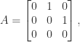
Satisfying these inequalities is not sufficient for positive definiteness. For example, the matrix

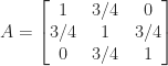
$A = \begin{bmatrix} 1 & 3/4 & 0 \\ 3/4 & 1 & 3/4 \\ 0 & 3/4 & 1 \\ \end{bmatrix}$

satisfies all the inequalities but $x^T\!Ax < 0$ for $x = [1,{}-\!\sqrt{2},~1]^T$ .

A sufficient condition for a symmetric matrix to be positive definite is that it has positive diagonal elements and is diagonally dominant, that is, 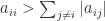$a_{ii} > \sum_{j \ne i} |a_{ij}|$ for all $i$ .

The definition requires the positivity of the quadratic form $x^T\!Ax$ . Sometimes this condition can be confirmed from the definition of $A$ . For example, if $A = B^T\!B$ and $B$ has linearly independent columns then $x^T\!Ax = (Bx)^T Bx > 0$ for $x\ne 0$ . Generally, though, this condition is not easy to check.

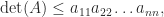
Two equivalent conditions to $A$ being symmetric positive definite are

every leading principal minor $\det(A_k)$ , where the submatrix $A_k = A(1\colon k, 1 \colon k)$ comprises the intersection of rows and columns $1$ to $k$ , is positive,
the eigenvalues of $A$ are all positive.

The first condition implies, in particular, that $\det(A) > 0$ , which also follows from the second condition since the determinant is the product of the eigenvalues.

Here are some other important properties of symmetric positive definite matrices.

$A^{-1}$ is positive definite.
$A$ has a unique symmetric positive definite square root $X$ , where a square root is a matrix $X$ such that $X^2 = A$ .
$A$ has a unique Cholesky factorization $A = R^T\!R$ , where $R$ is upper triangular with positive diagonal elements.

Sources of positive definite matrices include statistics, since nonsingular correlation matrices and covariance matrices are symmetric positive definite, and finite element and finite difference discretizations of differential equations.

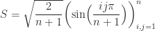
Examples of symmetric positive definite matrices, of which we display only the $4\times 4$ instances, are the Hilbert matrix

$H_4 = \left[\begin{array}{@{\mskip 5mu}c*{3}{@{\mskip 15mu} c}@{\mskip 5mu}} 1 & \frac{1}{2} & \frac{1}{3} & \frac{1}{4} \\[6pt] \frac{1}{2} & \frac{1}{3} & \frac{1}{4} & \frac{1}{5}\\[6pt] \frac{1}{3} & \frac{1}{4} & \frac{1}{5} & \frac{1}{6}\\[6pt] \frac{1}{4} & \frac{1}{5} & \frac{1}{6} & \frac{1}{7}\\[6pt] \end{array}\right],$

the Pascal matrix

$P_4 = \left[\begin{array}{@{\mskip 5mu}c*{3}{@{\mskip 15mu} r}@{\mskip 5mu}} 1 & 1 & 1 & 1\\ 1 & 2 & 3 & 4\\ 1 & 3 & 6 & 10\\ 1 & 4 & 10 & 20 \end{array}\right],$

and minus the second difference matrix, which is the tridiagonal matrix

$S_4 = \left[\begin{array}{@{\mskip 5mu}c*{3}{@{\mskip 15mu} r}@{\mskip 5mu}} 2 & -1 & & \\ -1 & 2 & -1 & \\ & -1 & 2 & -1 \\ & & -1 & 2 \end{array}\right].$

All three of these matrices have the property that $a_{ij}$ is non-decreasing along the diagonals. However, if $A$ is positive definite then so is $P^TAP$ for any permutation matrix $P$ , so any symmetric reordering of the row or columns is possible without changing the definiteness.

A $4\times 4$ symmetric positive definite matrix that was often used as a test matrix in the early days of digital computing is the Wilson matrix

$W = \begin{bmatrix} 5 &7& 6& 5 \\ 7 &10& 8& 7 \\ 6& 8& 10& 9 \\ 5& 7& 9 &10 \end{bmatrix}.$

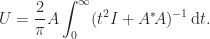
What is the best way to test numerically whether a symmetric matrix is positive definite? Computing the eigenvalues and checking their positivity is reliable, but slow. The fastest method is to attempt to compute a Cholesky factorization and declare the matrix positivite definite if the factorization succeeds. This is a reliable test even in floating-point arithmetic. If the matrix is not positive definite the factorization typically breaks down in the early stages so and gives a quick negative answer.

Symmetric block matrices

$C = \begin{bmatrix} A & X\\ X^T & B \end{bmatrix}$

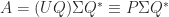
often appear in applications. If $A$ is nonsingular then we can write

$\begin{bmatrix} A & X\\ X^T & B \end{bmatrix} = \begin{bmatrix} I & 0\\ X^TA^{-1} & I \end{bmatrix} \begin{bmatrix} A & 0\\ 0 & B-X^TA^{-1}X \end{bmatrix} \begin{bmatrix} I & A^{-1}X\\ 0 & I \end{bmatrix},$

which shows that $C$ is congruent to a block diagonal matrix, which is positive definite when its diagonal blocks are. It follows that $C$ is positive definite if and only if both $A$ and $B - X^TA^{-1}X$ are positive definite. The matrix $B - X^TA^{-1}X$ is called the Schur complement of $A$ in $C$ .

We mention two determinantal inequalities. If the block matrix $C$ above is positive definite then $\det(C) \le \det(A) \det(B)$ (Fischer’s inequality). Applying this inequality recursively gives Hadamard’s inequality for a symmetric positive definite $A$ :

$\det(A) \le a_{11}a_{22} \dots a_{nn},$

with equality if and only if $A$ is diagonal.

Finally, we note that if $x^TAx \ge 0$ for all $x\ne0$ , so that the quadratic form is allowed to be zero, then the symmetric matrix $A$ is called symmetric positive semidefinite. Some, but not all, of the properties above generalize in a natural way. An important difference is that semidefinitness is equivalent to all principal minors, of which there are $2^{n-1}$ , being nonnegative; it is not enough to check the $n$ leading principal minors. Consider, as an example, the matrix

$\begin{bmatrix} 1 & 1 & 1\\ 1 & 1 & 1\\ 1 & 1 & 0 \end{bmatrix},$

which has leading principal minors $1$ , $0$ , and $0$ and a negative eigenvalue.

A complex $n\times n$ matrix $A$ is Hermitian positive definite if it is Hermitian ( $A$ is equal to its conjugate transpose, $A^*$ ) and $x^*Ax > 0$ for all nonzero vectors $x$ . Everything we have said above generalizes to the complex case.

References

This is a minimal set of references, which contain further useful references within.

Rajendra Bhatia, Positive Definite Matrices, Princeton University Press, Princeton, NJ, USA, 2007.
Nicholas J. Higham, Computing a nearest symmetric positive semidefinite matrix, Linear Algebra Appl. 103, 103–118, 1988. Section 5.
Roger A. Horn and Charles R. Johnson, Matrix Analysis, second edition, Cambridge University Press, 2013. My review of the second edition.

What Is the Growth Factor for Gaussian Elimination?

Gaussian elimination is the process of reducing an $n \times n$ matrix to upper triangular form by elementary row operations. It consists of $n$ stages, in the $k$ th of which multiples of row $k$ are added to later rows to eliminate elements below the diagonal in the $k$ th column. The result of Gaussian elimination (assuming it succeeds) is a factorization $A = LU$ , where $L$ is unit lower triangular (lower triangular with ones on the diagonal) and $U$ is upper triangular. This factorization reduces the solution of a linear system $Ax = b$ to the solution of two triangular systems.

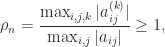
James Wilkinson showed in the early 1960s that the numerical stability of Gaussian elimination depends on the growth factor

$\rho_n = \displaystyle\frac{\max_{i,j,k} |a_{ij}^{(k)}|} {\max_{i,j}|a_{ij}|} \ge 1,$

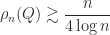
where the $a_{ij}^{(k)}$ are the elements at the start of the $k$ th stage of Gaussian elimination, with $A = \bigl(a_{ij}^{(1)}\bigr)$ . Specifically, he obtained a bound for the backward error of the computed solution that is proportional to $\rho_nu$ , where $u$ is the unit roundoff of the floating-point arithmetic. Wilkinson’s analysis focused attention on the size of the growth factor.

If no row interchanges are done during the elimination then $\rho_n$ can be arbitrarily large, as is easily seen for $n = 2$ . For some specific types of matrix more can be said.

If $A$ is symmetric positive definite then $\rho_n = 1$ . In this case one would normally use Cholesky factorization instead of LU factorization.
If $A$ is nonsingular and totally nonnegative (every submatrix has nonnegative determinant) then $\rho_n = 1$ .
If $A$ is diagonally dominant by rows or columns then $\rho_n \le 2$ .
If $A$ is complex and its real and imaginary parts are both symmetric positive definite then $\rho_n < 3$ .

The entry in the $(k,k)$ position at the start of stage $k$ of Gaussian elimination is called the pivot. By swapping rows and columns, any element with row and column indices greater than or equal to $k$ can be brought into the pivot position and used as the pivot. A pivoting strategy is a strategy for interchanging rows and columns at the start of each stage in order to choose a good sequence of pivots. For dense matrices the main criterion is that the pivoting strategy keeps the growth factor small, while for sparse matrices minimizing fill-in (a zero entry becoming nonzero) is also important.

Partial Pivoting

Partial pivoting interchanges rows to ensure that the pivot element is the largest in magnitude in its column. Wilkinson showed that partial pivoting ensures $\rho_n \le 2^{n-1}$ and that equality is attained for matrices of the form illustrated for $n = 4$ by

$\left[\begin{array}{@{\mskip3mu}rrrr} 1 & 0 & 0 & 1 \\ -1 & 1 & 0 & 1 \\ -1 & -1 & 1 & 1 \\ -1 & -1 & -1 & 1 \\ \end{array} \right].$

This matrix is a special case of a larger class of matrices for which equality is attained (Higham and Higham, 1989). Exponential growth can occur for matrices arising in practical applications, as shown by Wright for the multiple shooting method for two-point boundary value problems and Foster for a quadrature method for solving Volterra integral equations. Remarkably, though, $\rho_n$ is usually of modest size in practice. Explaining this phenomenon is one of the outstanding problems in numerical analysis.

Rook Pivoting

Rook pivoting interchanges rows and columns to ensure that the pivot element is the largest in magnitude in both its row and its column. Foster has shown that

$\rho_n \le 1.5 n^{\frac{3}{4} \log n}.$

This bound grows much more slowly than the bound for partial pivoting, but it can still be large. In practice, the bound is pessimistic.

Complete Pivoting

Complete pivoting chooses as pivot the largest element in magnitude in the remaining part of the matrix. Wilkinson (1961) showed that

$\rho_n \le n^{1/2} (2\cdot 3^{1/2} \cdots n^{1/(n-1)})^{1/2} \sim c \, n^{1/2} n^{\frac{1}{4}\log n}.$

This bound grows much more slowly than that for rook pivoting, but again it is pessimistic. Wilkinson noted in 1965 that no matrix had been discovered for which $\rho_n > n$ . Much interest has focused on the question of whether growth of $n$ can be exceeded and what is the largest possible growth. For a Hadamard matrix, $\rho_n \ge n$ , but such matrices do not exist for all $n$ . Evidence suggests that the growth factor for complete pivoting on a Hadamard matrix is exactly $n$ , and this has been proved for $n = 12$ and $n = 16$ .

That $\rho_n > n$ is possible was shown in the early 1990s by Gould (in floating-point arithmetic) and Edelman (in exact point arithmetic), through a $13\times 13$ matrix with growth $13.02$ .

Growth Factor Bounds for Any Pivoting Strategy

While much attention has focused on investigating the growth factor for particular pivoting strategies, some results are known that provide growth factor lower bounds for any pivoting strategy. Higham and Higham (1989) obtained a result that implies that for the symmetric orthogonal matrix

$S = \sqrt{ \displaystyle\frac{2}{n+1} } \biggl( \sin\Bigl( \displaystyle\frac{ij\pi}{n+1} \Bigr) \biggr)_{i,j=1}^n$

the lower bound

$\rho_n(S)\ge \displaystyle\frac{n+1}{2}$

holds for any pivoting strategy. Recently, Higham, Higham, and Pranesh (2020) have shown that

$\rho_n(Q) \gtrsim \displaystyle\frac{n}{4\log n}$

with high probability for large $n$ when $Q$ is a random orthogonal matrix from the Haar distribution. They show that the same bound holds for matrices that have only one singular value different from $1$ and have singular vector matrices that are random orthogonal matrices from the Haar distribution. These “randsvd matrices” can be generated as gallery('randsvd',n,kappa,2) in MATLAB.

Experimentation

If you want to experiment with growth factors in MATLAB, you can use the function gep from the Matrix Computation Toolbox. Examples:

>> rng(0); A = randn(1000);
>> [L,U,P,Q,rho] = gep(A,'p'); rho  % Partial pivoting.
rho =
   1.9437e+01
>> [L,U,P,Q,rho] = gep(A,'r'); rho  % Rook pivoting.
rho =
   9.9493e+00
>> [L,U,P,Q,rho] = gep(A,'c'); rho  % Complete pivoting.
rho =
   6.8363e+00
>> A = gallery('randsvd',1000,1e1,2);
>> [L,U,P,Q,rho] = gep(A,'c'); rho  % Complete pivoting.
rho =
   5.4720e+01

References

This is a minimal set of references, which contain further useful references within.

Alan Edelman, The complete pivoting conjecture for Gaussian elimination is false, The Mathematica Journal 2, 58–61, 1992.
Leslie V. Foster, The growth factor and efficiency of Gaussian elimination with rook pivoting, J. Comput. Appl. Math. 86, 177–194, 1997
Nicholas J. Higham and Desmond J. Higham, Large growth factors in Gaussian elimination with pivoting, SIAM J. Matrix Anal. Appl. 10 (2), 155–164, 1989.
Desmond J. Higham, Nicholas J. Higham, and Srikara Pranesh, Random Matrices Generating Large Growth in LU Factorization with Pivoting, MIMS EPrint 2020.13, The University of Manchester, UK, May 2020.
Nicholas J. Higham, Accuracy and Stability of Numerical Algorithms, second edition, Society for Industrial and Applied Mathematics, Philadelphia, PA, USA, 2002. Sections 9.4, 10.4.
Christos Kravvaritis and Marilena Mitrouli, The growth factor of a Hadamard matrix of order $16$ is $16$ , Numer. Linear Algebra Appl. 16, 715–743, 2009.
J. H. Wilkinson, Error analysis of direct methods of matrix inversion, J. Assoc. Comput. Mach. 8, 281–330, 1961.

What Is Stochastic Rounding?

In finite precision arithmetic the result of an elementary arithmetic operation does not generally lie in the underlying number system, $F$ , so it must be mapped back into $F$ by the process called rounding. The most common choice is round to nearest, whereby the nearest number in $F$ to the given number is chosen; this is the default in IEEE standard floating-point arithmetic.

Round to nearest is deterministic: given the same number it always produces the same result. A form of rounding that randomly rounds to the next larger or next smaller number was proposed Barnes, Cooke-Yarborough, and Thomas (1951), Forysthe (1959), and Hull and Swenson (1966). Now called stochastic rounding, it comes in two forms. The first form rounds up or down with equal probability $1/2$ .

We focus here on the second form of stochastic rounding, which is more interesting. To describe it we let $x\notin F$ be the given number and let $x_1$ and $x_2$ with $x_1 < x_2$ be the adjacent numbers in $F$ that are the candidates for the result of rounding. The following diagram shows the situation where $x$ lies just beyond the half-way point between $x_1$ and $x_2$ :

We round up to $x_2$ with probability $(x-x_1)/(x_2-x_1)$ and down to $x_1$ with probability $(x_2-x)/(x_2-x_1)$ ; note that these probabilities sum to $1$ . The probability of rounding to $x_1$ and $x_2$ is proportional to one minus the relative distance from $x$ to each number.

If stochastic rounding chooses to round to $x_1$ in the diagram then it has committed a larger error than round to nearest, which rounds to $x_2$ . Indeed if we focus on floating-point arithmetic then the result of the rounding is

$\mathrm{f\kern.2ptl}(x) = x (1+\delta), \quad |\delta|\le 2u,$

where $u$ is the unit roundoff. For round to nearest the same result is true with the smaller bound $|\delta|\le u$ . In addition, certain results that hold for round to nearest, such as 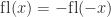$\mathrm{f\kern.2ptl}(x) = -\mathrm{f\kern.2ptl}(-x)$ and $\mathrm{f\kern.2ptl}(x/\sqrt{x^2+y^2}) \le 1$ , can fail for stochastic rounding. What, then, is the benefit of stochastic rounding?

It is not hard to show that the expected value of the result of stochastically rounding $x$ is $x$ itself (this is obvious if $x = (x_1+x_2)/2$ , for example), so the expected error is zero. Hence stochastic rounding maintains, in a statistical sense, some of the information that is discarded by a deterministic rounding scheme. This property leads to some important benefits, as we now explain.

In certain situations, round to nearest produces correlated rounding errors that cause systematic error growth. This can happen when we form the inner product of two long vectors $x$ and $y$ of nonnegative elements. If the elements all lie on $[0,1]$ then clearly the partial sum can grow monotonically as more and more terms are accumulated until at some point all the remaining terms “drop off the end” of the computed sum and do not change it—the sum stagnates. This phenomenon was observed and analyzed by Huskey and Hartree as long ago as 1949 in solving differential equations on the ENIAC. Stochastic rounding avoids stagnation by rounding up rather than down some of the time. The next figure gives an example. Here, $x$ and $y$ are $n$ -vectors sampled from the uniform $[0,1]$ distribution, the inner product is computed in IEEE standard half precision floating-point arithmetic ( $u \approx 4.9\times 10^{-4}$ ), and the backward errors are plotted for increasing $n$ . From about $n = 1000$ , the errors for stochastic rounding (SR, in orange) are smaller than those for round to nearest (RTN, in blue), the latter quickly reaching 1.

The figure is explained by recent results of Connolly, Higham, and Mary (2020). The key property is that the rounding errors generated by stochastic rounding are mean independent (a weaker version of independence). As a consequence, an error bound proportional to $\sqrt{n}u$ can be shown to hold with high probability. With round to nearest we have only the usual worst-case error bound, which is proportional to $nu$ . In the figure above, the solid black line is the standard backward error bound $nu$ while the dashed black line is $\sqrt{n}u$ . In this example the error with round to nearest is not bounded by a multiple of $\sqrt{n}u$ , as the blue curve crosses the dashed black one. The underlying reason is that the rounding errors for round to nearest are correlated (they are all negative beyond a certain point in the sum), whereas those for stochastic rounding are uncorrelated.

Another notable property of stochastic rounding is that the expected value of the computed inner product is equal to the exact inner product. The same is true more generally for matrix–vector and matrix–matrix products and the solution of triangular systems.

Stochastic rounding is proving popular in neural network training and inference when low precision arithmetic is used, because it avoids stagnation.

Implementing stochastic rounding efficiently is not straightforward, as the definition involves both a random number and an accurate value of the result that we are trying to compute. Possibilities include modifying low level arithmetic routines (Hopkins et al., 2020) and exploiting the augmented operations in the latest version of the IEEE standard floating-point arithmetic (Fasi and Mikaitis, 2020).

Hardware is starting to become available that supports stochastic rounding, including the Intel Lohi neuromorphic chip, the Graphcore Intelligence Processing Unit (intended to accelerate machine learning), and the SpiNNaker2 chip.

Stochastic rounding can be done in MATLAB using the chop function written by me and Srikara Pranesh. This function is intended for experimentation rather than efficient computation.

References

This is a minimal set of references, which contain further useful references within.

R. C. M. Barnes, E. H. Cooke-Yarborough, and D. G. A. Thomas, An electronic digital computor using cold cathode counting tubes for storage, Electronic Eng. 23, 286–291, 1951.
Michael P. Connolly, Nicholas J. Higham and Theo Mary, Stochastic Rounding and Its Probabilistic Backward Error Analysis, MIMS EPrint 2020.12, The University of Manchester, UK, April 2020.
Massimiliano Fasi and Mantas Mikaitis, Algorithms for Stochastically Rounded Elementary Arithmetic Operations in IEEE 754 Floating-Point Arithmetic, MIMS EPrint 2020.9, The University of Manchester, UK, February 2020.
George Forsythe, Reprint of a note on rounding-off errors, SIAM Rev. 1(1), 66–67, 1959.
Suyog Gupta and Ankur Agrawal and Kailash Gopalakrishnan and Pritish Narayanan, Deep Learning with Limited Numerical Precision, in Proceedings of the 32nd International Conference on International Conference on Machine Learning – Volume 37, ICML’15, JMLR.org, 2015, pp. 1737–1746,
Michael Hopkins, Mantas Mikaitis, Dave Lester, and Steve Furber, Stochastic rounding and reduced-precision fixed-point arithmetic for solving neural ordinary differential equations, Phil. Trans. R. Soc. A 378 (2166), 1–22, 2020.
T. E. Hull and J. R. Swenson, Tests of probabilistic models for propagation of roundoff errors, Comm. ACM 9 (3), 108–113, 1966.

Month: July 2020

What is the Polar Decomposition?

References

Related Blog Posts

Footnotes:

What Is a Symmetric Positive Definite Matrix?

References

Related Blog Posts

What Is the Growth Factor for Gaussian Elimination?

Partial Pivoting

Rook Pivoting

Complete Pivoting

Growth Factor Bounds for Any Pivoting Strategy

Experimentation

References

Related Blog Posts

What Is Stochastic Rounding?

References

Related Blog Posts

References

Related Blog Posts

Footnotes:

Share this:

References

Related Blog Posts

Share this:

Partial Pivoting

Rook Pivoting

Complete Pivoting

Growth Factor Bounds for Any Pivoting Strategy

Experimentation

References

Related Blog Posts

Share this:

References

Related Blog Posts

Share this: