A matrix is a rectangular array of numbers treated as a single object. A block matrix is a matrix whose elements are themselves matrices, which are called submatrices. By allowing a matrix to be viewed at different levels of abstraction, the block matrix viewpoint enables elegant proofs of results and facilitates the development and understanding of numerical algorithms.
A block matrix is defined in terms of a partitioning, which breaks a matrix into contiguous pieces. The most common and important case is for an 


![\notag A = \left[\begin{array}{cc|cc} a_{11} & a_{12} & a_{13} & a_{14}\\ a_{21} & a_{22} & a_{23} & a_{24}\\\hline a_{31} & a_{32} & a_{33} & a_{34}\\ a_{41} & a_{42} & a_{43} & a_{44}\\ \end{array}\right] = \begin{bmatrix} A_{11} & A_{12} \\ A_{21} & A_{22} \end{bmatrix},](https://s0.wp.com/latex.php?latex=%5Cnotag+++A+%3D+%5Cleft%5B%5Cbegin%7Barray%7D%7Bcc%7Ccc%7D+++++++++a_%7B11%7D+%26+a_%7B12%7D+%26+a_%7B13%7D+%26+a_%7B14%7D%5C%5C+++++++++a_%7B21%7D+%26+a_%7B22%7D+%26+a_%7B23%7D+%26+a_%7B24%7D%5C%5C%5Chline+++++++++a_%7B31%7D+%26+a_%7B32%7D+%26+a_%7B33%7D+%26+a_%7B34%7D%5C%5C+++++++++a_%7B41%7D+%26+a_%7B42%7D+%26+a_%7B43%7D+%26+a_%7B44%7D%5C%5C+++++++++%5Cend%7Barray%7D%5Cright%5D++++%3D++%5Cbegin%7Bbmatrix%7D+++++++++A_%7B11%7D+%26+A_%7B12%7D+%5C%5C+++++++++A_%7B21%7D+%26+A_%7B22%7D++++++++%5Cend%7Bbmatrix%7D%2C+&bg=ffffff&fg=222222&s=0&c=20201002)
where
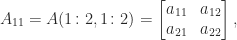
and similarly for the other blocks. The diagonal blocks in a partitioning of a square matrix are usually square (but not necessarily so), and they do not have to be of the same dimensions. This same 
![\notag A = \left[\begin{array}{c|ccc} a_{11} & a_{12} & a_{13} & a_{14}\\\hline a_{21} & a_{22} & a_{23} & a_{24}\\ a_{31} & a_{32} & a_{33} & a_{34}\\ a_{41} & a_{42} & a_{43} & a_{44}\\ \end{array}\right] = \begin{bmatrix} A_{11} & A_{12} \\ A_{21} & A_{22} \end{bmatrix},](https://s0.wp.com/latex.php?latex=%5Cnotag+++A+%3D+%5Cleft%5B%5Cbegin%7Barray%7D%7Bc%7Cccc%7D+++++++++a_%7B11%7D+%26+a_%7B12%7D+%26+a_%7B13%7D+%26+a_%7B14%7D%5C%5C%5Chline+++++++++a_%7B21%7D+%26+a_%7B22%7D+%26+a_%7B23%7D+%26+a_%7B24%7D%5C%5C+++++++++a_%7B31%7D+%26+a_%7B32%7D+%26+a_%7B33%7D+%26+a_%7B34%7D%5C%5C+++++++++a_%7B41%7D+%26+a_%7B42%7D+%26+a_%7B43%7D+%26+a_%7B44%7D%5C%5C+++++++++%5Cend%7Barray%7D%5Cright%5D++++%3D++%5Cbegin%7Bbmatrix%7D+++++++++A_%7B11%7D+%26+A_%7B12%7D+%5C%5C+++++++++A_%7B21%7D+%26+A_%7B22%7D++++++++%5Cend%7Bbmatrix%7D%2C+&bg=ffffff&fg=222222&s=0&c=20201002)
where 


The sum 


The product 


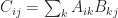


as long as all the eight products
Block matrix notation is an essential tool in numerical linear algebra. Here are some examples of its usage.
Matrix Factorization
For an 


The first row and column of 


The same type of construction applies to other factorizations, such as Cholesky factorization, QR factorization, and the Schur decomposition.
Matrix Inverse
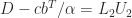
A useful formula for the inverse of a nonsingular block triangular matrix
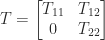
is
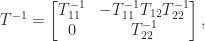
which has the special case
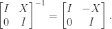
If 


We note that 
Determinantal Formulas
Block matrices provides elegant proofs of many results involving determinants. For example, consider the equations

which hold for any 


Constructing Matrices with Required Properties
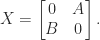
We can sometimes build a matrix with certain desired properties by a block construction. For example, if 


is a (block triangular) 

is involutory.
The Anti Block Diagonal Trick
For
Note that

Using these properties one can show a relation between the matrix sign function and the principal matrix square root:
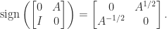
This allows one to derive iterations for computing the matrix square root and its inverse from iterations for computing the matrix sign function.
It is easy to derive explicit formulas for all the powers of
![\notag \mathrm{e}^X = \left[\begin{array}{cc} \cosh\sqrt{AB} & A (\sqrt{BA})^{-1} \sinh \sqrt{BA} \\[\smallskipamount] B(\sqrt{AB})^{-1} \sinh \sqrt{AB} & \cosh\sqrt{BA} \end{array}\right],](https://s0.wp.com/latex.php?latex=%5Cnotag+++%5Cmathrm%7Be%7D%5EX+%3D+%5Cleft%5B%5Cbegin%7Barray%7D%7Bcc%7D+++++++++++++++++++%5Ccosh%5Csqrt%7BAB%7D+%26+A+%28%5Csqrt%7BBA%7D%29%5E%7B-1%7D+%5Csinh+%5Csqrt%7BBA%7D++++++++++++++++++++++++%5C%5C%5B%5Csmallskipamount%5D+++++++++++++++++++++++B%28%5Csqrt%7BAB%7D%29%5E%7B-1%7D+%5Csinh+%5Csqrt%7BAB%7D+%26++++++++++++++++++++++%5Ccosh%5Csqrt%7BBA%7D++++++++++++++++++%5Cend%7Barray%7D%5Cright%5D%2C+&bg=ffffff&fg=222222&s=0&c=20201002)
where 


The most well known instance of the trick is when 

are plus and minus the singular values of 

References
This is a minimal set of references, which contain further useful references within.
- Gene Golub and Charles F. Van Loan, Matrix Computations, fourth edition, Johns Hopkins University Press, Baltimore, MD, USA, 2013.
- Nicholas J. Higham, Functions of Matrices: Theory and Computation, Society for Industrial and Applied Mathematics, Philadelphia, PA, USA, 2008. (Sections 1.5 and 1.6 for the theory of matrix square roots.)
- Roger A. Horn and Charles R. Johnson, Matrix Analysis, second edition, Cambridge University Press, 2013. My review of the second edition.
Related Blog Posts
This article is part of the “What Is” series, available from https://nhigham.com/category/what-is and in PDF form from the GitHub repository https://github.com/higham/what-is.
