Bfloat16 is a floating-point number format proposed by Google. The name stands for “Brain Floating Point Format” and it originates from the Google Brain artificial intelligence research group at Google.
Bfloat16 is a 16-bit, base 2 storage format that allocates 8 bits for the significand and 8 bits for the exponent. It contrasts with the IEEE fp16 (half precision) format, which allocates 11 bits for the significand but only 5 bits for the exponent. In both cases the implicit leading bit of the significand is not stored, hence the “+1” in this diagram:

The motivation for bfloat16, with its large exponent range, was that “neural networks are far more sensitive to the size of the exponent than that of the mantissa” (Wang and Kanwar, 2019).
Bfloat16 uses the same number of bits for the exponent as the IEEE fp32 (single precision) format. This makes conversion between fp32 and bfloat16 easy (the exponent is kept unchanged and the significand is rounded or truncated from 24 bits to 8) and the possibility of overflow in the conversion is largely avoided. Overflow can still happen, though (depending on the rounding mode): the significand of fp32 is longer, so the largest fp32 number exceeds the largest bfloat16 number, as can be seen in the following table. Here, the precision of the arithmetic is measured by the unit roundoff, which is 

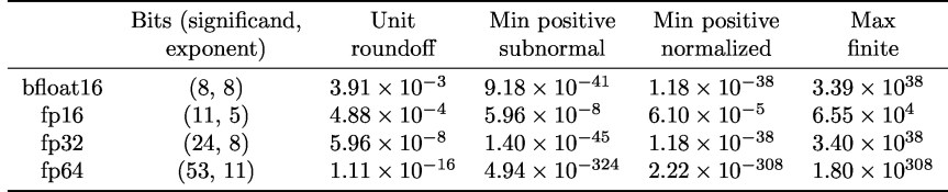
Note that although the table shows the minimum positive subnormal number for bfloat16, current implementations of bfloat16 do not appear to support subnormal numbers (this is not always clear from the documentation).
As the unit roundoff values in the table show, bfloat16 numbers have the equivalent of about three decimal digits of precision, which is very low compared with the eight and sixteen digits, respectively, of fp32 and fp64 (double precision).
The next table gives the number of numbers in the bfloat16, fp16, and fp32 systems. It shows that the bfloat16 number system is very small compared with fp32, containing only about 65,000 numbers.

The spacing of the bfloat16 numbers is large far from 1. For example, 65280, 65536, and 66048 are three consecutive bfloat16 numbers.
At the time of writing, bfloat16 is available, or announced, on four platforms or architectures.
- The Google Tensor Processing Units (TPUs, versions 2 and 3) use bfloat16 within the matrix multiplication units. In version 3 of the TPU the matrix multiplication units carry out the multiplication of 128-by-128 matrices.
- The NVIDIA A100 GPU, based on the NVIDIA Ampere architecture, supports bfloat16 in its tensor cores through block fused multiply-adds (FMAs)
with 8-by-8
and 8-by-4
.
- Intel has published a specification for bfloat16 and how it intends to implement it in hardware. The specification includes an FMA unit that takes as input two bfloat16 numbers
and
and an fp32 number
and computes
at fp32 precision, returning an fp32 number.
- The Arm A64 instruction set supports bfloat16. In particular, it includes a block FMA
The pros and cons of bfloat16 arithmetic versus IEEE fp16 arithmetic are
- bfloat16 has about one less (roughly three versus four) digit of equivalent decimal precision than fp16,
- bfloat16 has a much wider range than fp16, and
- current bfloat16 implementations do not support subnormal numbers, while fp16 does.
If you wish to experiment with bfloat16 but do not have access to hardware that supports it you will need to simulate it. In MATLAB this can be done with the chop function written by me and Srikara Pranesh.
References
This is a minimal set of references, which contain further useful references within.
- Arm A64 Instruction Set Architecture Armv8, for Armv8-A Architecture Profile, ARM Limited, 2019.
- Intel Corporation, BFLOAT16—Hardware Numerics Definition, 2018.
- IEEE Standard for Floating-Point Arithmetic, IEEE Std 754-2019 (Revision of IEEE 754-2008), The Institute of Electrical and Electronics Engineers, New York, 2019.
- NVIDIA Corporation, NVIDIA A100 Tensor Core GPU Architecture, 2020.
Related Blog Posts
- BFloat16 Processing for Neural Networks on Armv8-A by Nigel Stephens (2019)
- BFloat16: The Secret To High Performance on Cloud TPUs by Shibo Wang and Pankaj Kanwar (2019)
- A Multiprecision World (2017)
- Half Precision Arithmetic: fp16 Versus bfloat16 (2018)
- The Rise of Mixed Precision Arithmetic (2015)
- Simulating Low Precision Floating-Point Arithmetics in MATLAB (2020)
- What Is Floating-Point Arithmetic? (2020)
- What Is IEEE Standard Arithmetic? (2020)
This article is part of the “What Is” series, available from https://nhigham.com/category/what-is and in PDF form from the GitHub repository https://github.com/higham/what-is.
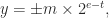
![e\in [e_{\min},e_{\max}]](https://s0.wp.com/latex.php?latex=e%5Cin+%5Be_%7B%5Cmin%7D%2Ce_%7B%5Cmax%7D%5D&bg=ffffff&fg=222222&s=0&c=20201002) is the exponent. The significand
is the exponent. The significand  is an integer satisfying
  . Numbers with
  are called normalized. Subnormal numbers, for which
  and
and  , are supported.
 .
.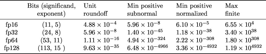 Fp32 (single precision) and fp64 (double precision) were in the 1985 standard; fp16 (half precision) and fp128 (quadruple precision) were introduced in 2008. Fp16 is defined only as a storage format, though it is widely used for computation.
 (usually written as inf in programing languages) as floating-point numbers: every arithmetic operation produces a number in the system. A NaN is generated by operations such as

 evaluates as
  when
when  .
.
 denotes the computed result. The standard also includes a fused multiply-add operation (FMA),
  . The definition requires it to be computed with just one rounding error, so that
  is the rounded version of
  , and hence satisfies
 ) and transcendental functions (
 ,
,  ,
,  ,
,  , etc.) and defines domains and special values for them, but these functions are not required.
 along with the error
  , for
, for  . These operations are useful for implementing compensated summation and other special high accuracy algorithms.
 . This has led to the development of an alternative 16-bit format that trades precision for range. The
  , smallest positive (subnormal) number xmins, smallest normalized positive number xmin, and largest finite number xmax for the three formats.
 . The series diverges, but when summed in the natural order in floating-point arithmetic it converges, because the partial sums grow while the addends decrease and eventually the addend is small enough that it does not change the partial sum. Here is a table showing the computed sum of the harmonic series for different precisions, along with how many terms are added before the sum becomes constant.


 . We are now seeing growing use of mixed precision, in which different floating point precisions are combined in order to deliver a result of the required accuracy at minimal cost.
 , is good enough for training and running neural networks. Here are some of the ways in which extra precision is currently being used.
 and
and  be distinct floating point numbers. How small can the relative difference between
  and
and  , which is called the unit roundoff.
  , where the infinity norm is
  ? It does not seem to be well known that
  can be much less than
  .
.  is possible.
  -vectors of normalized floating point numbers.
 for all
  such that
  .
.
