I thought it would be useful to provide my own MATLAB function nearcorr.m implementing the alternating projections algorithm. The listing is below. To see how it compares with the NAG code g02aa.m I ran the test code
%NEARCORR_TEST  Compare g02aa and nearcorr.

rng(10)                                  % Seed random number generators.
n = 100;
A = gallery('randcorr',n);               % Random correlation matrix.
E  = randn(n)*1e-1;  A = A + (E + E')/2; % Perturb it.
tol = 1e-10;

% A = cor1399; tol = 1e-4;

fprintf('g02aa:\n')
maxits = int64(-1);  % For linear equation solver.
maxit = int64(-1);   % For Newton iteration.
tic
[~,X1,iter1,feval,nrmgrd,ifail] = g02aa(A,'errtol',tol,'maxits',maxits, ...
                                          'maxit',maxit);
toc

fprintf('  Newton steps taken: %d\n', iter1);
fprintf('  Norm of gradient of last Newton step: %6.4f\n', nrmgrd);
if ifail > 0, fprintf('  g02aa failed with ifail = %g\n', ifail), end

fprintf('nearcorr:\n')
tic
[X2,iter2] = nearcorr(A,tol,[],[],[],[],1);
toc
fprintf('  Number of iterations: %d\n', iter2);

fprintf('  Normwise relative difference between computed solutions:')
fprintf('%9.2e\n', norm(X1-X2,1)/norm(X1,1))
Running under Windows 7 on an Ivy Bridge Core i7 processor @4.4Ghz I obtained the following results, where the “real-life” matrix is based on stock data:
| Matrix |
Code |
Time (secs) |
Iterations |
| 1. Random (100), tol = 1e-10 |
g02aa |
0.023 |
4 |
|
nearcorr |
0.052 |
15 |
| 2. Random (500), tol = 1e-10 |
g02aa |
0.48 |
4 |
|
nearcorr |
3.01 |
26 |
| 3. Real-life (1399), tol = 1e-4 |
g02aa |
6.8 |
5 |
|
nearcorr |
100.6 |
68 |
The results show that while nearcorr can be fast for small dimensions, the number of iterations, and hence its run time, tends to increase with the dimension and it can be many times slower than the Newton method. This is a stark illustration of the difference between quadratic convergence and linear (with problem-dependent constant) convergence. Here is my MATLAB function nearcorr.m.
function [X,iter] = nearcorr(A,tol,flag,maxits,n_pos_eig,w,prnt)
%NEARCORR    Nearest correlation matrix.
%   X = NEARCORR(A,TOL,FLAG,MAXITS,N_POS_EIG,W,PRNT)
%   finds the nearest correlation matrix to the symmetric matrix A.
%   TOL is a convergence tolerance, which defaults to 16*EPS.
%   If using FLAG == 1, TOL must be a 2-vector, with first component
%   the convergence tolerance and second component a tolerance
%   for defining "sufficiently positive" eigenvalues.
%   FLAG = 0: solve using full eigendecomposition (EIG).
%   FLAG = 1: treat as "highly non-positive definite A" and solve
%             using partial eigendecomposition (EIGS).
%   MAXITS is the maximum number of iterations (default 100, but may
%   need to be increased).
%   N_POS_EIG (optional) is the known number of positive eigenvalues of A.
%   W is a vector defining a diagonal weight matrix diag(W).
%   PRNT = 1 for display of intermediate output.

%   By N. J. Higham, 13/6/01, updated 30/1/13, 15/11/14, 07/06/15.
%   Reference:  N. J. Higham, Computing the nearest correlation
%   matrix---A problem from finance. IMA J. Numer. Anal.,
%   22(3):329-343, 2002.

if ~isequal(A,A'), error('A must by symmetric.'), end
if nargin < 2 || isempty(tol), tol = length(A)*eps*[1 1]; end
if nargin < 3 || isempty(flag), flag = 0; end
if nargin < 4 || isempty(maxits), maxits = 100; end
if nargin < 6 || isempty(w), w = ones(length(A),1); end
if nargin < 7, prnt = 1; end

n = length(A);
if flag >= 1
   if nargin < 5 || isempty(n_pos_eig)
      [V,D] = eig(A); d = diag(D);
      n_pos_eig = sum(d >= tol(2)*d(n));
   end
   if prnt, fprintf('n = %g, n_pos_eig = %g\n', n, n_pos_eig), end
end

X = A; Y = A;
iter = 0;
rel_diffX = inf; rel_diffY = inf; rel_diffXY = inf;
dS = zeros(size(A));

w = w(:); Whalf = sqrt(w*w');

while max([rel_diffX rel_diffY rel_diffXY]) > tol(1)

   Xold = X;
   R = Y - dS;
   R_wtd = Whalf.*R;
   if flag == 0
      X = proj_spd(R_wtd);
   elseif flag == 1
      [X,np] = proj_spd_eigs(R_wtd,n_pos_eig,tol(2));
   end
   X = X ./ Whalf;
   dS = X - R;
   Yold = Y;
   Y = proj_unitdiag(X);
   rel_diffX = norm(X-Xold,'fro')/norm(X,'fro');
   rel_diffY = norm(Y-Yold,'fro')/norm(Y,'fro');
   rel_diffXY = norm(Y-X,'fro')/norm(Y,'fro');
   iter = iter + 1;
   if prnt
      fprintf('%2.0f:  %9.2e  %9.2e  %9.2e', ...
               iter, rel_diffX, rel_diffY, rel_diffXY)
      if flag >= 1, fprintf('  np = %g\n',np), else fprintf('\n'), end
   end
   if iter > maxits
       error(['Stopped after ' num2str(maxits) ' its. Try increasing MAXITS.'])
   end

end

%%%%%%%%%%%%%%%%%%%%%%%%
function A = proj_spd(A)
%PROJ_SPD

if ~isequal(A,A'), error('Not symmetric!'), end
[V,D] = eig(A);
A = V*diag(max(diag(D),0))*V';
A = (A+A')/2; % Ensure symmetry.

%%%%%%%%%%%%%%%%%%%%%%%%%%%%%%%%%%%%%%%%%%%%%%%%%%%%%%%%%%%%%
function [A,n_pos_eig_found] = proj_spd_eigs(A,n_pos_eig,tol)
%PROJ_SPD_EIGS

if ~isequal(A,A'), error('Not symmetric!'), end
k = n_pos_eig + 10; % 10 is safety factor.
if k > length(A), k = n_pos_eig; end
opts.disp = 0;
[V,D] = eigs(A,k,'LA',opts); d = diag(D);
j = (d > tol*max(d));
n_pos_eig_found = sum(j);
A = V(:,j)*D(j,j)*V(:,j)';  % Build using only the selected eigenpairs.
A = (A+A')/2; % Ensure symmetry.

%%%%%%%%%%%%%%%%%%%%%%%%%%%%%
function A = proj_unitdiag(A)
%PROJ_SPD

n = length(A);
A(1:n+1:n^2) = 1;
Updates
- Links updated August 4, 2014.
nearcorr.m corrected November 15, 2014: iter was incorrectly initialized (thanks to Mike Croucher for pointing this out).- Added link to Mike Croucher’s Python alternating directions code, November 17, 2014.
- Corrected an error in the convergence test, June 7, 2015. Effect on performance will be minimal (thanks to Nataša Strabić for pointing this out).


![\notag A = \begin{bmatrix} 1 & \frac{1}{2} & \frac{1}{3} & \frac{1}{4} \\[3pt] \frac{1}{2} & 1 & \frac{2}{3} & \frac{1}{2} \\[3pt] \frac{1}{3} & \frac{2}{3} & 1 & \frac{3}{4} \\[3pt] \frac{1}{4} & \frac{1}{2} & \frac{3}{4} & 1 \end{bmatrix}.](https://s0.wp.com/latex.php?latex=%5Cnotag+++A+%3D+%5Cbegin%7Bbmatrix%7D+++++++++1+++++++++++%26+%5Cfrac%7B1%7D%7B2%7D++%26+%5Cfrac%7B1%7D%7B3%7D+%26+%5Cfrac%7B1%7D%7B4%7D+%5C%5C%5B3pt%5D+++++++++%5Cfrac%7B1%7D%7B2%7D+%26+++++++++++1++%26+%5Cfrac%7B2%7D%7B3%7D+%26+%5Cfrac%7B1%7D%7B2%7D+%5C%5C%5B3pt%5D+++++++++%5Cfrac%7B1%7D%7B3%7D+%26++%5Cfrac%7B2%7D%7B3%7D+%26+1+++++++++++%26+%5Cfrac%7B3%7D%7B4%7D+%5C%5C%5B3pt%5D+++++++++%5Cfrac%7B1%7D%7B4%7D+%26++%5Cfrac%7B1%7D%7B2%7D+%26+%5Cfrac%7B3%7D%7B4%7D+%26++1+++++++++%5Cend%7Bbmatrix%7D.+&bg=ffffff&fg=222222&s=0&c=20201002)


-Factorizations with Small Pivots, Math. Comp. 42(166), 535–547, 1984.
 are column vectors with
  elements, each vector containing samples of a random variable, then the corresponding
  has
has 
 is the mean of the elements in
  . If
. If  has nonzero diagonal elements then we can scale the diagonal to 1 to obtain the corresponding correlation matrix
 . The
. The 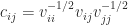 is the correlation between the variables
  .
.![[-1, 1]](https://s0.wp.com/latex.php?latex=%5B-1%2C+1%5D&bg=ffffff&fg=222222&s=0&c=20201002) .
.![[0,n]](https://s0.wp.com/latex.php?latex=%5B0%2Cn%5D&bg=ffffff&fg=222222&s=0&c=20201002) .
. (since the eigenvalues of a matrix sum to its trace).
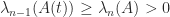
 ,
,  ,
,  . The only value of
  and
and  that makes
  with every off-diagonal element equal to
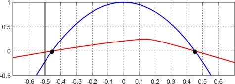
  , illustrated for
  by
by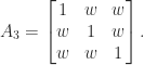
 .
. , so we solve the problem
 remain fixed. And we may want to weight some elements more than others, by using a weighted Frobenius norm. These are convex optimization problems and have a unique solution that can be computed using the alternating projections method (Higham, 2002) or a Newton algorithm (Qi and Sun, 2006; Borsdorf and Higham, 2010).
 , where
  is a target correlation matrix (Higham, Strabić, and Šego, 2016). Shrinking can readily incorporate fixed blocks and weighting.
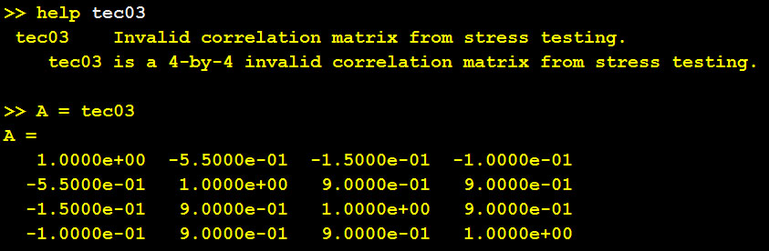
 I learned about Anderson acceleration in the minisymposium