What makes the matrix sign function so interesting and useful is that it can be computed directly without first computing eigenvalues or eigenvectore of  . Roberts noted that the iteration

converges quadratically to  . This iteration is Newton’s method applied to the equation
  , with starting matrix . It is one of the rare circumstances in which explicitly inverting matrices is justified!
Various other iterations are available for computing . A matrix multiplication-based iteration is the Newton–Schulz iteration

This iteration is quadratically convergent if  for some subordinate matrix norm. The Newton–Schulz iteration is the
 ![[1/0]](https://s0.wp.com/latex.php?latex=%5B1%2F0%5D&bg=ffffff&fg=222222&s=0&c=20201002) member of a Padé family of rational iterations
member of a Padé family of rational iterations

where  is the
 ![[\ell/m]](https://s0.wp.com/latex.php?latex=%5B%5Cell%2Fm%5D&bg=ffffff&fg=222222&s=0&c=20201002) Padé approximant to
Padé approximant to  (
( and
and  are polynomials of degrees at most
  and
and  , respectively). The iteration is globally convergent to for
  and
and  , and for
  it converges when , with order of convergence
  in all cases.
Although the rate of convergence of these iterations is at least quadratic, and hence asymptotically fast, it can be slow initially. Indeed for  , if
, if  then the Newton iteration computes
 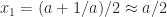 , and so the early iterations make slow progress towards
  . Fortunately, it is possible to speed up convergence with the use of scale parameters. The Newton iteration can be replaced by
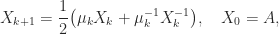
with, for example,
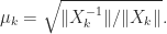
This parameter  can be computed at no extra cost.
As an example, we took A = gallery('lotkin',4), which has eigenvalues  ,
,  ,
,  , and
, and  to four significant figures. After six iterations of the unscaled Newton iteration
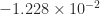
  had an eigenvalue
  , showing that is far from , which has eigenvalues . Yet when scaled by (using the
  -norm), after six iterations all the eigenvalues of
  were within distance
  of , and the iteration had converged to within this tolerance.
The Matrix Computation Toolbox contains a MATLAB function signm that computes the matrix sign function. It computes a Schur decomposition then obtains the sign of the triangular Schur factor by a finite recurrence. This function is too expensive for use in applications, but is reliable and is useful for experimentation.

 generate a sequence of points
  , where the step from
  is along a search direction
  determined from a linear system
  , where
  is the gradient and
  is an approximation to the Hessian matrix
  . The equation
  shows that
  , and in order to guarantee that this condition holds for all
  , where
  is a permutation matrix,
  is unit lower triangular, and
  is diagonal or block diagonal and positive definite. It follows that
  is a positive definite matrix.
 to
to  . However, choosing a suitable
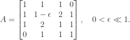
 are the square roots of the pivots. After one step of elimination the reduced matrix is
![\notag A^{(2)} = \left[\begin{array}{c|ccc} 1 & 1 & 1 & 1\\\hline 0 & -\epsilon & 1 & 1\\ 0 & 1 & 0 & 1\\ 0 & 1 & 1 & 1 \end{array}\right],](https://s0.wp.com/latex.php?latex=%5Cnotag+++A%5E%7B%282%29%7D+%3D+++%5Cleft%5B%5Cbegin%7Barray%7D%7Bc%7Cccc%7D++++1+%26+1++++++++++%26+1+%26+1%5C%5C%5Chline++++0+%26+-%5Cepsilon+%26++1+++%26+1%5C%5C++++0+%26++1++++++++++%26+0+%26+1%5C%5C++++0+%26+++1+++++++++%26+1+%26+1+++%5Cend%7Barray%7D%5Cright%5D%2C+&bg=ffffff&fg=222222&s=0&c=20201002)
 matrix (a Schur complement) is clearly indefinite because the
  entry, which is the next pivot, is negative. We can make the (2,2) entry positive by adding
  to it:
![\notag A^{(2)} + E = \left[\begin{array}{c|ccc} 1 & 1 & 1 & 1\\\hline 0 & \epsilon & 1 & 1\\ 0 & 1 & 0 & 1\\ 0 & 1 & 1 & 1 \end{array}\right] \quad (E = 2 \mskip1mu\epsilon \mskip1mu e_2e_2^T).](https://s0.wp.com/latex.php?latex=%5Cnotag+++A%5E%7B%282%29%7D+%2B+E+%3D+++%5Cleft%5B%5Cbegin%7Barray%7D%7Bc%7Cccc%7D++++1+%26+1++++++++++%26+1+%26+1%5C%5C%5Chline++++0+%26+%5Cepsilon+%26+1+++%26+1%5C%5C++++0+%26+1+++++++++++%26+0+%26+1%5C%5C++++0+%26+1+++++++++++%26+1+%26+1+++%5Cend%7Barray%7D%5Cright%5D+++%5Cquad+++%28E+%3D++2+%5Cmskip1mu%5Cepsilon+%5Cmskip1mu+e_2e_2%5ET%29.+&bg=ffffff&fg=222222&s=0&c=20201002)
![\notag A^{(3)} = \left[\begin{array}{cc|cc} 1 & 1 & 1 & 1 \\ 0 & \epsilon & 1 & 1 \\\hline\rule{0cm}{18pt} 0 & 0 & -\displaystyle\frac{1}{\epsilon} & 1 - \displaystyle\frac{1}{\epsilon}\\\rule{0cm}{20pt} 0 & 0 &1 - \displaystyle\frac{1}{\epsilon} & 1 - \displaystyle\frac{1}{\epsilon} \end{array}\right],](https://s0.wp.com/latex.php?latex=%5Cnotag+++A%5E%7B%283%29%7D+%3D+++%5Cleft%5B%5Cbegin%7Barray%7D%7Bcc%7Ccc%7D++++1+%26+1++++++++++%26+1+%26+1+%5C%5C++++0+%26+%5Cepsilon+++%26+1+%26+1+%5C%5C%5Chline%5Crule%7B0cm%7D%7B18pt%7D++++0+%26+0++++++++++%26+-%5Cdisplaystyle%5Cfrac%7B1%7D%7B%5Cepsilon%7D+%26+1+-+%5Cdisplaystyle%5Cfrac%7B1%7D%7B%5Cepsilon%7D%5C%5C%5Crule%7B0cm%7D%7B20pt%7D++++0+%26+0++++++++++%261+-+%5Cdisplaystyle%5Cfrac%7B1%7D%7B%5Cepsilon%7D+%26++1+-+%5Cdisplaystyle%5Cfrac%7B1%7D%7B%5Cepsilon%7D+++%5Cend%7Barray%7D%5Cright%5D%2C+&bg=ffffff&fg=222222&s=0&c=20201002)
 submatrix has elements of order
  . Not only will a perturbation of order
  be required to the
  element to allow the Cholesky factorization to continue, but the Cholesky factor will have elements of order
  so numerical stability will likely be lost. Yet the smallest eigenvalue of
  perturbation to
  is not much larger than

 flops for an
  matrix.
 factorization
  , were
  . The pivoting strategy is the symmetric rook pivoting strategy of Ashcraft, Grimes, and Lewis (1998), which has the key property of producing a bounded
  comparisons but can be as large as
  in the worst case. Cheng and Higham compute the perturbation
  of minimal Frobenius norm such that
  has eigenvalues greater than or equal to
  , where
  is a parameter. The modified Cholesky factorization is then
  .
. matrix above with
  :
: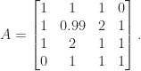
 (where
  is the unit roundoff), the perturbed matrix
  ,
,  , and
, and  , respectively, and the 2-norm condition numbers are
  ,
,  , and
, and  . The large condition number for the Cheng–Higham algorithm is caused by the value of the parameter
  , the perturbed matrix is
 from
from  . For comparison, the symmetric matrix with all eigenvalues greater than or equal to
  that is closest to
  from
from 
 is a Jordan decomposition with
  then
then
 are therefore all
  , so
, so  and
and  are projectors onto the invariant subspaces associated with the eigenvalues of
  , with the eigenvalues of
  in the open left half-plane and those of
  in the open right half-plane (
 ). Then
![X = [X_1~X_2]](https://s0.wp.com/latex.php?latex=X+%3D+%5BX_1%7EX_2%5D&bg=ffffff&fg=222222&s=0&c=20201002) , where
, where  is
is  and
and  is
is  , we have
![\notag \begin{aligned} \displaystyle\frac{I+S}{2} &= X \begin{bmatrix} 0 & 0 \\ 0 & I_q \end{bmatrix}X^{-1} = X_2 X^{-1}(p+1\colon n,:),\\[\smallskipamount] \displaystyle\frac{I-S}{2} &= X \begin{bmatrix} I_p & 0 \\ 0 & 0 \end{bmatrix}X^{-1} = X_1 X^{-1}(1\colon p,:). \end{aligned}](https://s0.wp.com/latex.php?latex=%5Cnotag+%5Cbegin%7Baligned%7D+++%5Cdisplaystyle%5Cfrac%7BI%2BS%7D%7B2%7D+%26%3D+X+%5Cbegin%7Bbmatrix%7D+0+%26+0+%5C%5C++++++++++++++++++++++++++++++++++++++++++++++++0+++%26+I_q+++++++++++%5Cend%7Bbmatrix%7DX%5E%7B-1%7D+%3D+X_2+X%5E%7B-1%7D%28p%2B1%5Ccolon+n%2C%3A%29%2C%5C%5C%5B%5Csmallskipamount%5D+++%5Cdisplaystyle%5Cfrac%7BI-S%7D%7B2%7D+%26%3D+X+%5Cbegin%7Bbmatrix%7D+I_p+%26+0+%5C%5C++++++++++++++++++++++++++++++++++++++++++++++++++0+++%26+0+++++++++++%5Cend%7Bbmatrix%7DX%5E%7B-1%7D+%3D+X_1+X%5E%7B-1%7D%281%5Ccolon+p%2C%3A%29.+%5Cend%7Baligned%7D+&bg=ffffff&fg=222222&s=0&c=20201002)


 block of the equation
 and
and  then
then
![\bigl[\begin{smallmatrix}A & -C\\ 0& B \end{smallmatrix}\bigr]](https://s0.wp.com/latex.php?latex=%5Cbigl%5B%5Cbegin%7Bsmallmatrix%7DA+%26+-C%5C%5C+0%26+B+%5Cend%7Bsmallmatrix%7D%5Cbigr%5D&bg=ffffff&fg=222222&s=0&c=20201002) . The conditions that
. The conditions that  are identity matrices are satisfied for the Lyapunov equation
  when
when  , where
  and
and  are Hermitian.
 satisfies
  , where
  and
and  are the number of eigenvalues in the open left-half plane and open right-half plane, respectively (as above). Since
  , we have the formulas
 and
and  with
with  ,
,
 . Formulas also exist to count the number of eigenvalues in rectangles and more complicated regions.
![\notag \mathrm{sign}\left( \begin{bmatrix} 0 & A \\\ I & 0 \end{bmatrix} \right ) = \begin{bmatrix}0 & A^{1/2} \\ A^{-1/2} & 0 \end{bmatrix}, \\[\smallskipamount]](https://s0.wp.com/latex.php?latex=%5Cnotag+++++%5Cmathrm%7Bsign%7D%5Cleft%28+%5Cbegin%7Bbmatrix%7D+0+%26+A+%5C%5C%5C+I+%26+0+%5Cend%7Bbmatrix%7D+%5Cright+%29++++++%3D+%5Cbegin%7Bbmatrix%7D0+%26+A%5E%7B1%2F2%7D+%5C%5C+A%5E%7B-1%2F2%7D+%26+0+%5Cend%7Bbmatrix%7D%2C+%5C%5C%5B%5Csmallskipamount%5D+&bg=ffffff&fg=222222&s=0&c=20201002)

 is a polar decomposition. Among other things, these relations yield iterations for
  and
and  by applying the iterations above to the relevant block
  matrix and reading off the (1,2) block.
 , and it can be written
  . For a rational number
  (where
  and
and  are integers), defining
  is more difficult: is it
  or
or  ? These two possibilities can be different even for
  for an arbitrary real number
  ?
? we define
  , where
  is the principal logarithm: the one taking values in the strip
  . We can generalize this definition to matrices. For a nonsingular matrix
 lie in the strip
 ![\alpha \in [-1,1]](https://s0.wp.com/latex.php?latex=%5Calpha+%5Cin+%5B-1%2C1%5D&bg=ffffff&fg=222222&s=0&c=20201002) , the eigenvalues of
, the eigenvalues of  where
where  is an eigenvalue of
  of the complex plane.
 for a positive integer

 is called the principal
 can be a different matrix. In general, it is not true that
  for real
  , although for symmetric positive definite matrices this identity does hold because the eigenvalues are real and positive.
 is
is
 with
with  is given by the binomial expansion
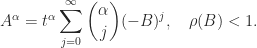

 there is an explicit formula for
  , where
  . Let
. Let  and
and  . It can be shown that
 can be used computationally, but it is somewhat indirect in that one must approximate both the exponential and the logarithm. A more direct algorithm based on the Schur decomposition and Padé approximation of the power function is developed by Higham and Lin (2013). MATLAB code is available from
  for some nonsingular
  , then
  . This formula is safe to use computationally only if
  then
then  , by the definition of square root. If
  does it follow that
  ? Clearly, the answer is “no” in general because, for example,
  does not imply
  .
. for
for  is the inverse function of
  for
for ![\alpha\in[-1,1]](https://s0.wp.com/latex.php?latex=%5Calpha%5Cin%5B-1%2C1%5D&bg=ffffff&fg=222222&s=0&c=20201002) .
. ? For
? For  , but for real
  such that
  . Assume that
  . Hence the normwise relative backward error is
![\notag \eta(X) = \displaystyle\frac{ \|X^{1/\alpha} - A \|}{\|A\|}, \quad \alpha\in[-1,1].](https://s0.wp.com/latex.php?latex=%5Cnotag++++++%5Ceta%28X%29+%3D+%5Cdisplaystyle%5Cfrac%7B+%5C%7CX%5E%7B1%2F%5Calpha%7D+-+A+%5C%7C%7D%7B%5C%7CA%5C%7C%7D%2C+%5Cquad+%5Calpha%5Cin%5B-1%2C1%5D.+&bg=ffffff&fg=222222&s=0&c=20201002)
 element is the probability of moving from state
  to state
  (years to months) and
  (weeks to days) are among the values of interest. Unfortunately,
 ![\notag A = \left[\begin{array}{ccc} 0 & 1 & 0\\ 0 & 0 & 1\\ 1 & 0 & 0\\ \end{array} \right]](https://s0.wp.com/latex.php?latex=%5Cnotag++++A+%3D+%5Cleft%5B%5Cbegin%7Barray%7D%7Bccc%7D++++++++0++%26+1+%26+0%5C%5C++++++++0++%26+0+%26+1%5C%5C++++++++1++%26+0+%26+0%5C%5C++++++++%5Cend%7Barray%7D+%5Cright%5D+&bg=ffffff&fg=222222&s=0&c=20201002)
![\notag A^{1/2} = \frac{1}{3} \left[\begin{array}{rrr} 2 & 2 & -1 \\ -1 & 2 & 2 \\ 2 & -1 & 2 \end{array} \right],](https://s0.wp.com/latex.php?latex=%5Cnotag++++A%5E%7B1%2F2%7D+%3D+%5Cfrac%7B1%7D%7B3%7D+%5Cleft%5B%5Cbegin%7Barray%7D%7Brrr%7D++++++++2++%26+2+%26+-1+%5C%5C++++++++-1+%26+2+%26+2+%5C%5C++++++++2+%26+-1+%26+2++++++++%5Cend%7Barray%7D+%5Cright%5D%2C+&bg=ffffff&fg=222222&s=0&c=20201002)
![\notag Y = \left[\begin{array}{ccc} 0 & 0 & 1\\ 1 & 0 & 0\\ 0 & 1 & 0\\ \end{array} \right]](https://s0.wp.com/latex.php?latex=%5Cnotag+++++++++Y+%3D+%5Cleft%5B%5Cbegin%7Barray%7D%7Bccc%7D++++++++++0++%26+0++%26++1%5C%5C++++++++++1++%26+0++%26++0%5C%5C++++++++++0++%26+1++%26++0%5C%5C++++++++++%5Cend%7Barray%7D+%5Cright%5D+&bg=ffffff&fg=222222&s=0&c=20201002)
 !)
!)
 , for all
 for some
  with
with  for
for  and
and  ,
,  . Kingman showed in 1962 that this condition holds if and only if for every positive integer
  such that
  .
. , in which case for large problems it is preferable to directly approximate
  or
or  for all
  . Here, the square root is the principal square root (the one lying in the right half-plane) and the logarithm is the principal logarithm (the one with imaginary part in
 ![(-\pi,\pi]](https://s0.wp.com/latex.php?latex=%28-%5Cpi%2C%5Cpi%5D&bg=ffffff&fg=222222&s=0&c=20201002) ).
). by
by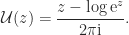
 , in that
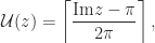
 is the ceiling function, which returns the smallest integer greater than or equal to its argument. It follows that
  if and only if
 ![\mathrm{Im} z \in (-\pi, \pi]](https://s0.wp.com/latex.php?latex=%5Cmathrm%7BIm%7D+z+%5Cin+%28-%5Cpi%2C+%5Cpi%5D&bg=ffffff&fg=222222&s=0&c=20201002) . Hence
. Hence  , replacing
  in
in  ), we have
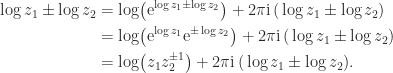

 , in which each occurrence of
  , we have
![\notag f\left( \begin{bmatrix} \lambda_1 & t_{12} \\ 0 & \lambda_2 \end{bmatrix} \right) = \begin{bmatrix} f(\lambda_1) & t_{12} f[\lambda_1,\lambda_2] \\ 0 & f(\lambda_2) \end{bmatrix},](https://s0.wp.com/latex.php?latex=%5Cnotag+++++f%5Cleft%28+%5Cbegin%7Bbmatrix%7D++++++++++++++++++++++%5Clambda_1+%26+t_%7B12%7D++%5C%5C++++++++++++++++++++++++++++0+++%26+%5Clambda_2+++++++++++++%5Cend%7Bbmatrix%7D+%5Cright%29++++++++++%3D+%5Cbegin%7Bbmatrix%7D+++++++++++++++f%28%5Clambda_1%29+%26+t_%7B12%7D+f%5B%5Clambda_1%2C%5Clambda_2%5D+%5C%5C+++++++++++++++++0++++++++++%26+f%28%5Clambda_2%29+++++++++++++%5Cend%7Bbmatrix%7D%2C+&bg=ffffff&fg=222222&s=0&c=20201002)
![\notag f[\lambda_1,\lambda_2] = \begin{cases} \displaystyle\frac{f(\lambda_2)-f(\lambda_1)}{\lambda_2-\lambda_1}, & \lambda_1 \ne \lambda_2, \\ f'(\lambda_1), & \lambda_1 = \lambda_2. \end{cases}](https://s0.wp.com/latex.php?latex=%5Cnotag+++f%5B%5Clambda_1%2C%5Clambda_2%5D++++%3D+%5Cbegin%7Bcases%7D++++++%5Cdisplaystyle%5Cfrac%7Bf%28%5Clambda_2%29-f%28%5Clambda_1%29%7D%7B%5Clambda_2-%5Clambda_1%7D%2C++++++%26+%5Clambda_1+%5Cne+%5Clambda_2%2C+%5C%5C++++++f%27%28%5Clambda_1%29%2C+%26+%5Clambda_1+%3D+%5Clambda_2.+++++%5Cend%7Bcases%7D+&bg=ffffff&fg=222222&s=0&c=20201002)
 this formula suffers from numerical cancellation. For the logarithm, we can rewrite it, using
  , as
, as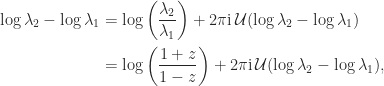
 . Using the hyperbolic arc tangent, defined by
![\notag f[\lambda_1,\lambda_2] = \displaystyle\frac{2\mathrm{atanh}(z) + 2\pi \mathrm{i}\, \mathcal{U}(\log \lambda_2 - \log \lambda_1)}{\lambda_2-\lambda_1}, \quad \lambda_1 \ne \lambda_2.](https://s0.wp.com/latex.php?latex=%5Cnotag+++f%5B%5Clambda_1%2C%5Clambda_2%5D++++%3D+%5Cdisplaystyle%5Cfrac%7B2%5Cmathrm%7Batanh%7D%28z%29+%2B+2%5Cpi+%5Cmathrm%7Bi%7D%5C%2C++++++%5Cmathcal%7BU%7D%28%5Clog+%5Clambda_2+-+%5Clog+%5Clambda_1%29%7D%7B%5Clambda_2-%5Clambda_1%7D%2C++++%5Cquad+%5Clambda_1+%5Cne+%5Clambda_2.+&bg=ffffff&fg=222222&s=0&c=20201002)
 function this formula will provide an accurate value of
 ![f[\lambda_1,\lambda_2]](https://s0.wp.com/latex.php?latex=f%5B%5Clambda_1%2C%5Clambda_2%5D&bg=ffffff&fg=222222&s=0&c=20201002) provided that
provided that  by
by
 if and only if the imaginary parts of all the eigenvalues of
 ![(-\pi, \pi]](https://s0.wp.com/latex.php?latex=%28-%5Cpi%2C+%5Cpi%5D&bg=ffffff&fg=222222&s=0&c=20201002) . Furthermore,
. Furthermore,  is a diagonalizable matrix with integer eigenvalues.
![\notag A = \left[\begin{array}{rrrr} 3 & 1 & -1 & -9\\ -1 & 3 & 9 & -1\\ -1 & -9 & 3 & 1\\ 9 & -1 & -1 & 3 \end{array}\right], \quad \Lambda(A) = \{ 2\pm 8\mathrm{i}, 4 \pm 10\mathrm{i} \}](https://s0.wp.com/latex.php?latex=%5Cnotag+++A+%3D+%5Cleft%5B%5Cbegin%7Barray%7D%7Brrrr%7D++++3+%26+1+%26+-1+%26+-9%5C%5C++++-1+%26+3+%26+9+%26+-1%5C%5C++++-1+%26+-9+%26+3+%26+1%5C%5C++++9+%26+-1+%26+-1+%26+3+%5Cend%7Barray%7D%5Cright%5D%2C++++%5Cquad+%5CLambda%28A%29+%3D+%5C%7B+2%5Cpm+8%5Cmathrm%7Bi%7D%2C+4+%5Cpm+10%5Cmathrm%7Bi%7D+%5C%7D+&bg=ffffff&fg=222222&s=0&c=20201002)
![\notag X = \mathcal{U}(A) = \mathrm{i} \left[\begin{array}{rrrr} 0 & -\frac{1}{2} & 0 & \frac{3}{2}\\ \frac{1}{2} & 0 & -\frac{3}{2} & 0\\ 0 & \frac{3}{2} & 0 & -\frac{1}{2}\\ -\frac{3}{2} & 0 & \frac{1}{2} & 0 \end{array}\right], \quad \Lambda(X) = \{ \pm 1, \pm 2 \}.](https://s0.wp.com/latex.php?latex=%5Cnotag+++X+%3D+%5Cmathcal%7BU%7D%28A%29+%3D+%5Cmathrm%7Bi%7D+%5Cleft%5B%5Cbegin%7Barray%7D%7Brrrr%7D++++0+%26+-%5Cfrac%7B1%7D%7B2%7D+%26+0+%26+%5Cfrac%7B3%7D%7B2%7D%5C%5C++++%5Cfrac%7B1%7D%7B2%7D+%26+0+%26+-%5Cfrac%7B3%7D%7B2%7D+%26+0%5C%5C++++0+%26+%5Cfrac%7B3%7D%7B2%7D+%26+0+%26+-%5Cfrac%7B1%7D%7B2%7D%5C%5C++++-%5Cfrac%7B3%7D%7B2%7D+%26+0+%26+%5Cfrac%7B1%7D%7B2%7D+%26+0+%5Cend%7Barray%7D%5Cright%5D%2C++++%5Cquad+%5CLambda%28X%29+%3D+%5C%7B+%5Cpm+1%2C+%5Cpm+2+%5C%7D.+&bg=ffffff&fg=222222&s=0&c=20201002)
 .
. ,
,

 . If
. If ![\alpha\in(-1,1]](https://s0.wp.com/latex.php?latex=%5Calpha%5Cin%28-1%2C1%5D&bg=ffffff&fg=222222&s=0&c=20201002) and
and  then
then  and so
![\notag (A^\alpha)^{1/\alpha} = A, \quad \alpha \in [-1,1],](https://s0.wp.com/latex.php?latex=%5Cnotag++++++%28A%5E%5Calpha%29%5E%7B1%2F%5Calpha%7D+%3D+A%2C+%5Cquad+%5Calpha+%5Cin+%5B-1%2C1%5D%2C++++&bg=ffffff&fg=222222&s=0&c=20201002)
 , too.
 are nonsingular and
  then
then

![\arg\lambda_i + \arg\mu_i \in(-\pi,\pi]](https://s0.wp.com/latex.php?latex=%5Carg%5Clambda_i+%2B+%5Carg%5Cmu_i+%5Cin%28-%5Cpi%2C%5Cpi%5D&bg=ffffff&fg=222222&s=0&c=20201002) for every eigenvalue
for every eigenvalue  of
of  of
of  .
. ,
,

![(-\pi/2,\pi/2]](https://s0.wp.com/latex.php?latex=%28-%5Cpi%2F2%2C%5Cpi%2F2%5D&bg=ffffff&fg=222222&s=0&c=20201002) then
then  .
.
 , and this equation also holds for
![\mathrm{Im} \lambda \in(-\pi,\pi]](https://s0.wp.com/latex.php?latex=%5Cmathrm%7BIm%7D+%5Clambda+%5Cin%28-%5Cpi%2C%5Cpi%5D&bg=ffffff&fg=222222&s=0&c=20201002) . Using
. Using  in place of
  and
and  . See Aprahamian and Higham (2014) for details.
 ? In principle yes, but if the inverse is multivalued the answer is not immediate. The matrix unwinding function is useful for analyzing such round trip relations. As an example, if
  for an integer
 is the principal arc cosine defined in Aprahamian and Higham (2016), where this result and analogous results for the arc sine, arc hyperbolic cosine, and arc hyperbolic sine are derived; and
  is the matrix sign function.