In numerical linear algebra a blocked algorithm organizes a computation so that it works on contiguous chunks of data. A blocked algorithm and the corresponding unblocked algorithm (with blocks of size 
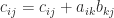
A simple example of blocking is in computing an inner product 

- for
-
- end


can be expressed in blocked form, with block size 
- for
-
% Compute by the unblocked algorithm.
- end


The sums of
To see the full benefits of blocking we need to consider an algorithm operating on matrices, of which matrix multiplication is the most important example. Suppose we wish to compute the product 


- for
- for
- for
-
- end
- end
- end


Let 


- for
- for
- for
-
- end
- end
- end


On a computer with a hierarchical memory the blocked form can be much more efficient than the point form if the blocks fit into the high speed memory, as much less data transfer is required. Indeed line 5 of the blocked algorithm performs 


The LAPACK (first released in 1992) was the first program library to systematically use blocked algorithms for a wide range of linear algebra computations.
An extra advantage that blocked algorithms have over unblocked algorithms is a reduction in the error constant in a rounding error bound by a factor
The adjective “block” is sometimes used in place of “blocked”, but we prefer to reserve “block” for the meaning described in the next section.
Block Algorithms
A block algorithm is a generalization of a scalar algorithm in which the basic scalar operations become matrix operations (


An example of a block factorization is block LU factorization. For a 
![\notag A = \left[ \begin{tabular}{cc|cc} 1 & & & \\ x & 1 & & \\ \hline x & x & 1 & \\ x & x & x & 1 \end{tabular} \right] \left[ \begin{tabular}{cc|cc} x & x & x & x \\ & x & x & x \\ \hline & & x & x \\ & & & x \end{tabular} \right].](https://s0.wp.com/latex.php?latex=%5Cnotag++++A+%3D++%5Cleft%5B+%5Cbegin%7Btabular%7D%7Bcc%7Ccc%7D++++++++++++++++++1+%26+++%26++++%26++++%5C%5C++++++++++++++++++x+%26+1+%26++++%26++++%5C%5C++%5Chline++++++++++++++++++x+%26+x+%26++1+%26++++%5C%5C++++++++++++++++++x+%26+x+%26++x+%26+1+++++++++++++++++%5Cend%7Btabular%7D++%5Cright%5D++++++%5Cleft%5B+%5Cbegin%7Btabular%7D%7Bcc%7Ccc%7D++++++++++++++++++x+%26+x+%26++x+%26+x++%5C%5C++++++++++++++++++++%26+x+%26++x+%26+x++%5C%5C++%5Chline++++++++++++++++++++%26+++%26++x+%26+x++%5C%5C++++++++++++++++++++%26+++%26++++%26+x+++++++++++++++++%5Cend%7Btabular%7D++%5Cright%5D.+&bg=ffffff&fg=222222&s=0&c=20201002)
A block LU factorization has the form
![\notag A = \left[ \begin{tabular}{cc|cc} 1 & 0 & & \\ 0 & 1 & & \\ \hline x & x & 1 & 0 \\ x & x & 0 & 1 \end{tabular} \right] \left[ \begin{tabular}{cc|cc} x & x & x & x \\ x & x & x & x \\ \hline & & x & x \\ & & x & x \end{tabular} \right].](https://s0.wp.com/latex.php?latex=%5Cnotag++++A+++%3D++%5Cleft%5B+%5Cbegin%7Btabular%7D%7Bcc%7Ccc%7D++++++++++++++++++1+%26+0+%26++++%26++++%5C%5C++++++++++++++++++0+%26+1+%26++++%26++++%5C%5C++%5Chline++++++++++++++++++x+%26+x+%26++1+%26+0++%5C%5C++++++++++++++++++x+%26+x+%26++0+%26+1+++++++++++++++++%5Cend%7Btabular%7D++%5Cright%5D++++++%5Cleft%5B+%5Cbegin%7Btabular%7D%7Bcc%7Ccc%7D++++++++++++++++++x+%26+x+%26++x+%26+x++%5C%5C++++++++++++++++++x+%26+x+%26++x+%26+x++%5C%5C++%5Chline++++++++++++++++++++%26+++%26++x+%26+x++%5C%5C++++++++++++++++++++%26+++%26++x+%26+x+++++++++++++++++%5Cend%7Btabular%7D++%5Cright%5D.+&bg=ffffff&fg=222222&s=0&c=20201002)
Clearly, these are different factorizations. In general, a block LU factorization has the form 


The adjective “block” also applies to a variety of matrix properties, for which there are often special-purpose block algorithms. For example, the matrix
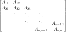
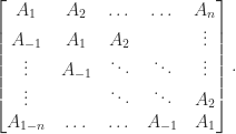
is a block tridiagonal matrix, and a block Toeplitz matrix has constant block diagonals:
One can define block diagonal dominance as a generalization of diagonal dominance. A block Householder matrix generalizes a Householder matrix: it is a perturbation of the identity matrix by a matrix of rank greater than or equal to
References
This is a minimal set of references, which contain further useful references within.
- Nicholas J. Higham, Accuracy and Stability of Numerical Algorithms, second edition, Society for Industrial and Applied Mathematics, Philadelphia, PA, USA, 2002. (Chapter 13, “Block LU Factorization”.)
- Nicholas J. Higham, Numerical Stability of Algorithms at Extreme Scale and Low Precisions, MIMS EPrint 2021.14, Manchester Institute for Mathematical Sciences, The University of Manchester, UK, September 2021.
Related Blog Posts
- Can We Solve Linear Algebra Problems at Extreme Scale and Low Precisions? (2021)
- What Is a Block Matrix? (2020)
- What Is an LU Factorization? (2021)
This article is part of the “What Is” series, available from https://nhigham.com/category/what-is and in PDF form from the GitHub repository https://github.com/higham/what-is.
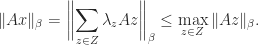
 satisfying
 with equality if and only if
  (nonnegativity),
 for all
  ,
,  (homogeneity),
 for all
  (the triangle inequality).
 the corresponding subordinate matrix norm on
  is defined by
 -, and
  -vector norms it can be shown that
 denotes the largest singular value of
  -norm no explicit formula is known for
  for
for  .
.

 , whereas
  for any subordinate norm), but it is consistent.
 for any unitary matrices
  . For the Frobenius norm the invariance follows easily from the trace formula.
 such that
  for
for  and any consistent matrix norm,
 is the spectral radius (the largest absolute value of any eigenvalue). To prove this inequality, let
  be an eigenvalue of
  the corresponding eigenvector (necessarily nonzero), and form the matrix
 ![X=[x,x,\dots,x] \in \mathbb{C}^{n\times n}](https://s0.wp.com/latex.php?latex=X%3D%5Bx%2Cx%2C%5Cdots%2Cx%5D+%5Cin+%5Cmathbb%7BC%7D%5E%7Bn%5Ctimes+n%7D&bg=ffffff&fg=222222&s=0&c=20201002) . Then
. Then  , so
, so  , giving
  since
since  . For a subordinate norm it suffices to take norms in the equation
  .
.
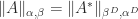
 , where the first two equalities are obtained from the singular value decomposition and we have used (1).
 .
. is given in the next result. Recall that
  denotes the dual of the vector norm
  .
.
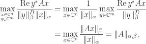
 . Here,
  denotes
  .
. .
.
 – and
– and  -norms to be the same
  , where
  (giving, in particular,
  and
and  , which are easily obtained directly).
 norm when
 ,
,


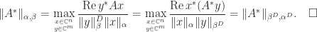
 , where the maximum is attained for
  . For (4), using the Hölder inequality,
 th row of
  .
. . The unit cube
  , where
 ![e = [1,1,\dots,1]^T](https://s0.wp.com/latex.php?latex=e+%3D+%5B1%2C1%2C%5Cdots%2C1%5D%5ET&bg=ffffff&fg=222222&s=0&c=20201002) , is a convex polyhedron, so any point within it is a convex combination of the vertices, which are the elements of
, is a convex polyhedron, so any point within it is a convex combination of the vertices, which are the elements of  . Hence
  implies
 , but trivially
  and (5) follows.
 . Then, using a Cholesky factorization
  (which exists even if
 we have
 . Hence
  , using (5).

 -norm has recently found use in statistics (Cape, Tang, and Priebe, 2019), the motivation being that because it satisfies
 and so can be a better norm to use in bounds. The
  -norms are used by Rebrova and Vershynin (2018) in bounding the
  and
and  random variables, respectively.
 ) norm is not consistent, but for any vector norm
  , we have
 . This class of matrices includes magic squares and doubly stochastic matrices. We have
  , so
, so  by (2). But
  for the vector
  of
of  by (1). Hence
  . In fact,
  for all
 ![p\in[1,\infty]](https://s0.wp.com/latex.php?latex=p%5Cin%5B1%2C%5Cinfty%5D&bg=ffffff&fg=222222&s=0&c=20201002) (see Higham (2002, Prob. 6.4) and Stoer and Witzgall (1962)).
(see Higham (2002, Prob. 6.4) and Stoer and Witzgall (1962)). ,
,  , or
, or  , for example, and we may wish to compute the norm without forming
  15.2). The power method accesses
  -norm and the
  -norm, which we compare with the
 ![p \in[1,25]](https://s0.wp.com/latex.php?latex=p+%5Cin%5B1%2C25%5D&bg=ffffff&fg=222222&s=0&c=20201002) . This shape of curve is typical, because, as the plot in the lower half indicates,
. This shape of curve is typical, because, as the plot in the lower half indicates,  is a convex function of
  for
for  (see Higham, 2002, Sec.
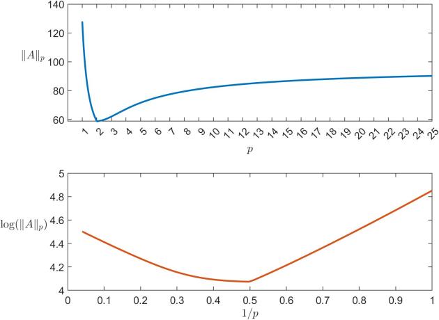
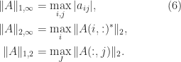
 norm, which is the max norm in (6), is investigated by Higham and Relton (2016) and extended to estimate the
  or
or  .
. can be defined by

 for all
  independent of
 ![[1.33,1.41]](https://s0.wp.com/latex.php?latex=%5B1.33%2C1.41%5D&bg=ffffff&fg=222222&s=0&c=20201002) , or
, or ![[1.67,1.79]](https://s0.wp.com/latex.php?latex=%5B1.67%2C1.79%5D&bg=ffffff&fg=222222&s=0&c=20201002) for the analogous inequality for real data. See Friedland, Lim, and Zhang (2018) and the references therein.
for the analogous inequality for real data. See Friedland, Lim, and Zhang (2018) and the references therein. is due to Rohn (2000), who shows that evaluating it is NP-hard. For general
