March 2022 – Nick Higham

The inverse of a matrix $A\in\mathbb{C}^{n\times n}$ is a matrix $X\in\mathbb{C}^{n\times n}$ such that $AX = I$ , where $I$ is the identity matrix (which has ones on the diagonal and zeros everywhere else). The inverse is written as $A^{-1}$ . If the inverse exists then $A$ is said to be nonsingular or invertible, and otherwise it is singular.

The inverse $X$ of $A$ also satisfies $XA = I$ , as we now show. The equation $AX = I$ says that $Ax_j = e_j$ for $j=1\colon n$ , where $x_j$ is the $j$ th column of $A$ and $e_j$ is the $j$ th unit vector. Hence the $n$ columns of $A$ span $\mathbb{C}^n$ , which means that the columns are linearly independent. Now $A(I-XA) = A - AXA = A -A = 0$ , so every column of $I - XA$ is in the null space of $A$ . But this contradicts the linear independence of the columns of $A$ unless $I - XA = 0$ , that is, $XA = I$ .

The inverse of a nonsingular matrix is unique. If $AX = AW = I$ then premultiplying by $X$ gives $XAX = XAW$ , or, since $XA = I$ , $X = W$ .

The inverse of the inverse is the inverse: $(A^{-1})^{-1} = A$ , which is just another way of interpreting the equations $AX = XA = I$ .

Connections with the Determinant

Since the determinant of a product of matrices is the product of the determinants, the equation $AX = I$ implies $\det(A) \det(X) = 1$ , so the inverse can only exist when $\det(A) \ne 0$ . In fact, the inverse always exists when $\det(A) \ne 0$ .

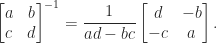
An explicit formula for the inverse is

$\notag A^{-1} = \displaystyle\frac{\mathrm{adj}(A)}{\det(A)}, \qquad (1)$

where the adjugate $\mathrm{adj}$ is defined by

$\bigl(\mathrm{adj}(A)\bigr)_{ij} = (-1)^{i+j} \det(A_{ji})$

and where $A_{pq}$ denotes the submatrix of $A$ obtained by deleting row $p$ and column $q$ . A special case is the formula

$\notag \begin{bmatrix} a & b \\ c& d \end{bmatrix}^{-1} = \displaystyle\frac{1}{ad-bc} \begin{bmatrix} d & -b \\ -c & a \end{bmatrix}.$

The equation $AA^{-1} = I$ implies $\det(A^{-1}) = 1/\det(A)$ .

Conditions for Nonsingularity

The following result collects some equivalent conditions for a matrix to be nonsingular. We denote by $\mathrm{null}(A)$ the null space of $A$ (also called the kernel).

Theorem 1. For $A \in \mathbb{C}^{n \times n}$ the following conditions are equivalent to $A$ being nonsingular:

$\mathrm{null}(A) = \{0\}$ ,

$\mathrm{rank}(A) = n$ ,

$Ax=b$ has a unique solution $x$ , for any $b$ ,

none of the eigenvalues of $A$ is zero,

$\det(A) \ne 0$ .

A useful formula is

$\notag (AB)^{-1} = B^{-1}A^{-1}.$

Here are some facts about the inverses of $n\times n$ matrices of special types.

A diagonal matrix $D = \mathrm{diag}(d_i)$ is nonsingular if $d_i\ne0$ for all $i$ , and $D^{-1} = \mathrm{diag}(d_i^{-1})$ .
An upper (lower) triangular matrix $T$ is nonsingular if its diagonal elements are nonzero, and the inverse is upper (lower) triangular with $(i,i)$ element $t_{ii}^{-1}$ .
If $x,y\in\mathbb{C}^n$ and $y^*A^{-1}x \ne -1$ , then $A + xy^*$ is nonsingular and
$\notag \bigl(A + xy^*\bigr)^{-1} = A^{-1} - \displaystyle\frac{A^{-1}x y^* A^{-1}}{1 + y^*A^{-1}x}.$

This is the Sherman–Morrison formula.

The Inverse as a Matrix Polynomial

The Cayley-–Hamilton theorem says that a matrix satisfies its own characteristic equation, that is, if $p(t) = \det(tI - A) = t^n + c_{n-1} t^{n-1} + \cdots + c_0$ , then $p(A) = 0$ . In other words, $A^n + c_{n-1} A^{n-1} + \cdots + c_0I = 0$ , and if $A$ is nonsingular then multiplying through by $A^{-1}$ gives (since $c_0 = p(0) = (-1)^n\det(A) \ne 0)$

$A^{-1} = -\displaystyle\frac{1}{c_0} (A^{n-1} + c_{n-1} A^{n-2} + \cdots + c_1 I). \qquad (2)$

This means that $A^{-1}$ is expressible as a polynomial of degree at most $n-1$ in $A$ (with coefficients that depend on $A$ ).

To Compute or Not to Compute the Inverse

The inverse is an important theoretical tool, but it is rarely necessary to compute it explicitly. If we wish to solve a linear system of equations $Ax = b$ then computing $A^{-1}$ and then forming $x = A^{-1}b$ is both slower and less accurate in floating-point arithmetic than using LU factorization (Gaussian elimination) to solve the system directly. Indeed, for $n = 1$ one would not solve $3x = 1$ by computing $3^{-1} \times 1$ .

For sparse matrices, computing the inverse may not even be practical, as the inverse is usually dense.

If one needs to compute the inverse, how should one do it? We will consider the cost of different methods, measured by the number of elementary arithmetic operations (addition, subtraction, division, multiplication) required. Using (1), the cost is that of computing one determinant of order $n$ and $n^2$ determinants of order $n-1$ . Since computing a $k\times k$ determinant costs at least $O(k^3)$ operations by standard methods, this approach costs at least $O(n^5)$ operations, which is prohibitively expensive unless $n$ is very small. Instead one can compute an LU factorization with pivoting and then solve the systems $Ax_i = e_i$ for the columns $x_i$ of $A^{-1}$ , at a total cost of $2n^3 + O(n^2)$ operations.

Equation (2) does not give a good method for computing $A^{-1}$ , because computing the coefficients $c_i$ and evaluating a matrix polynomial are both expensive.

It is possible to exploit fast matrix multiplication methods, which compute the product of two $n\times n$ matrices in $O(n^\alpha)$ operations for some $\alpha < 3$ . By using a block LU factorization recursively, one can reduce matrix inversion to matrix multiplication. If we use Strassen’s fast matrix multiplication method, which has $\alpha = \log_2 7 \approx 2.807$ , then we can compute $A^{-1}$ in $O(n^{2.807})$ operations.

Slash Notation

MATLAB uses the backslash and forward slash for “matrix division”, with the meanings $A \backslash B = A^{-1}B$ and $A / B = AB^{-1}$ . Note that because matrix multiplication is not commutative, $A \backslash B \ne A / B$ , in general. We have $A\backslash I = I/A = A^{-1}$ and $I\backslash A = A/I = A$ . In MATLAB, the inverse can be compute with inv(A), which uses LU factorization with pivoting.

Rectangular Matrices

If $A$ is $m\times n$ then the equation $AX = I_m$ requires $X$ to be $n\times m$ , as does $XA = I_n$ . Rank considerations show that at most one of these equations can hold if $m\ne n$ . For example, if $A = a^*$ is a nonzero row vector, then $AX = 1$ for $X = a/a^*a$ , but $XA = aa^*/a^*a\ne I$ . This is an example of a generalized inverse.

An Interesting Inverse

Here is a triangular matrix with an interesting inverse. This example is adapted from the LINPACK Users’ Guide, which has the matrix, with “LINPACK” replacing “INVERSE” on the front cover and the inverse on the back cover.

$\notag \left[\begin{array}{ccccccc} I & N & V & E & R & S & E\\ 0 & N & V & E & R & S & E\\ 0 & 0 & V & E & R & S & E\\ 0 & 0 & 0 & E & R & S & E\\ 0 & 0 & 0 & 0 & R & S & E\\ 0 & 0 & 0 & 0 & 0 & S & E\\ 0 & 0 & 0 & 0 & 0 & 0 & E \end{array}\right]^{-1} = \left[\begin{array}{*{7}{r@{\hspace{4pt}}}} 1/I & -1/I & 0 & 0 & 0 & 0 & 0\\ 0 & 1/N & -1/N & 0 & 0 & 0 & 0\\ 0 & 0 & 1/V & -1/V & 0 & 0 & 0\\ 0 & 0 & 0 & 1/E & -1/E & 0 & 0\\ 0 & 0 & 0 & 0 & 1/R & -1/R & 0\\ 0 & 0 & 0 & 0 & 0 & 1/S & -1/S\\ 0 & 0 & 0 & 0 & 0 & 0 & 1/E \end{array}\right].$

Related Blog Posts

What Is a Generalized Inverse? (2020)
What Is a Sparse Matrix? (2020)
What Is an LU Factorization? (2021)
What Is the Adjugate of a Matrix? (2020)
What Is the Determinant of a Matrix? (2021)
What Is the Sherman–Morrison–Woodbury Formula? (2020)

This article is part of the “What Is” series, available from https://nhigham.com/index-of-what-is-articles/ and in PDF form from the GitHub repository https://github.com/higham/what-is.

Square Matrix: $m = n$

When $A$ is square, backslash returns $x = A^{-1}b$ , computed by LU factorization with partial pivoting (and of course without forming $A^{-1}$ ). There is no special treatment for singular matrices, so for them division by zero may occur and the output may contain NaNs (in practice, what happens will usually depend on the rounding errors). For example:

>> A = [1 0; 0 0], b = [1 0]', x = A\b
A =
     1     0
     0     0
b =
     1
     0
Warning: Matrix is singular to working precision. 

x =
     1
   NaN

Backslash take advantage of various kinds of structure in $A$ ; see MATLAB Guide (section 9.3) or doc mldivide in MATLAB.

Overdetermined System: $m > n$

An overdetermined system has no solutions, in general. Backslash yields a least squares (LS) solution, which is unique if $A$ has full rank. If $A$ is rank-deficient then there are infinitely many LS solutions, and backslash returns a basic solution: one with at most $\mathrm{rank}(A)$ nonzeros. Such a solution is not, in general, unique.

Underdetermined System: $m < n$

An underdetermined system has fewer equations than unknowns, so either there is no solution of there are infinitely many. In the latter case $A\backslash b$ produces a basic solution and in the former case a basic LS solution. Example:

>> A = [1 1 1; 1 1 0]; b = [3 2]'; x = A\b
x =
   2.0000e+00
            0
   1.0000e+00

Another basic solution is $[0~2~1]^T$ , and the minimum $2$ -norm solution is $[1~1~1]^T$ .

A\A

Now we turn to the special case $A\backslash A$ , which in terms of equation (1) is a solution to $AX = A$ . If $A = 0$ then $X = I$ is not a basic solution, so $A\backslash A \ne I$ ; in fact, $0\backslash 0 = 0$ if $m\ne n$ and it is matrix of NaNs if $m = n$ .

For an underdetermined system with full-rank $A$ , $A\backslash A$ is not necessarily the identity matrix:

>> A = [1 0 1; 0 1 0], X = A\A
A =
     1     0     1
     0     1     0
X =
     1     0     1
     0     1     0
     0     0     0

But for an overdetermined system with full-rank $A$ , $A\backslash A$ is the identity matrix:

>> A'\A'
ans =
   1.0000e+00            0
  -1.9185e-17   1.0000e+00

Minimum Frobenius Norm Solution

The MATLAB definition of $A\backslash b$ is a pragmatic one, as it computes a solution or LS solution to $Ax = b$ in the most efficient way, using LU factorization ( $m = n$ ) or QR factorization $(m\ne n$ ). Often, one wants the solution of minimum $2$ -norm, which can be expressed as $A^+b$ , where $A^+$ is the pseudoinverse of $A$ . In MATLAB, $A^+b$ can be computed by lsqminnorm(A,b) or pinv(A)*b, the former expression being preferred as it avoids the unnecessary computation of $A^+$ and it uses a complete orthogonal factorization instead of an SVD.

When the right-hand side is a matrix, $B$ , lsqminnorm(A,B) and pinv(A)*B give the solution of minimal Frobenius norm, which we write as $A \backslash\backslash B$ . Then $A\backslash\backslash A = A^+A$ , which is the orthogonal projector onto $\mathrm{range}(A^*)$ , and it is equal to the identity matrix when $m\ge n$ and $A$ has full rank. For the matrix above:

>> A = [1 0 1; 0 1 0], X = lsqminnorm(A,A)
A =
     1     0     1
     0     1     0
X =
   5.0000e-01            0   5.0000e-01
            0   1.0000e+00            0
   5.0000e-01            0   5.0000e-01

Month: March 2022

What Is the Matrix Inverse?

Connections with the Determinant

Conditions for Nonsingularity

The Inverse as a Matrix Polynomial

To Compute or Not to Compute the Inverse

Slash Notation

Rectangular Matrices

An Interesting Inverse

Related Blog Posts

What Is A\A?

Square Matrix: $m = n$

Overdetermined System: $m > n$

Underdetermined System: $m < n$

A\A

Minimum Frobenius Norm Solution

Related Blog Posts

Connections with the Determinant

Conditions for Nonsingularity

The Inverse as a Matrix Polynomial

To Compute or Not to Compute the Inverse

Slash Notation

Rectangular Matrices

An Interesting Inverse

Related Blog Posts

Share this:

Square Matrix:

Overdetermined System:

Underdetermined System:

A\A

Minimum Frobenius Norm Solution

Related Blog Posts

Share this:

Square Matrix: $m = n$

Overdetermined System: $m > n$

Underdetermined System: $m < n$