What Is Gershgorin’s Theorem?

For a given $n\times n$ matrix, Gershgorin’s theorem defines $n$ discs in the complex plane whose union contains the eigenvalues of the matrix. The theorem can provide approximations to eigenvalues. It can also provide qualitative information, such as that all the eigenvalues lie in a particular half-plane.

Theorem 1 (Gershgorin’s theorem).

The eigenvalues of $A\in\mathbb{C}^{n\times n}$ lie in the union of the $n$ discs in the complex plane

$\notag D_i = \Big\{ z\in\mathbb{C}: |z-a_{ii}| \le \displaystyle\sum_{j\ne i} |a_{ij}|\Big\}, \quad i=1\colon n.$

Proof. Let $\lambda$ be an eigenvalue of $A$ and $x$ a corresponding eigenvector and let $|x_k| = \|x\|_\infty$ . From the $k$ th equation in $Ax=\lambda x$ we have

$\notag \sum_{j=1 \atop j\ne k}^n a_{kj}x_j = (\lambda-a_{kk}) x_k.$

Hence

$\notag |\lambda-a_{kk}| \le \sum_{j=1 \atop j\ne k}^n |a_{kj}||x_j|/|x_k|,$

and since $|x_j|/|x_k|\le 1$ it follows that $\lambda$ belongs to the $k$ th disc, $D_k$ .

The Gershgorin discs $D_i$ are defined in terms of a summation over the rows of $A$ , but since the eigenvalues of $A$ are the same as those of $A^T$ the same result holds with summation over the columns.

A consequence of the theorem is that if $0$ does not belong to any of the Gershgorin discs then $A$ is nonsingular. This is equivalent to the well-known result that a strictly diagonally dominant matrix is nonsingular.

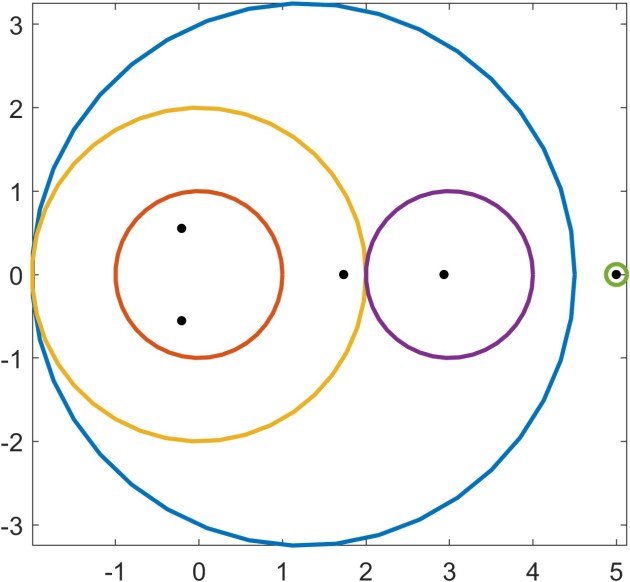
Another consequence of the theorem is that if $A$ is symmetric and all the discs lie in the open right half-plane then the eigenvalues are positive and so $A$ is positive definite. This condition is equivalent to $A$ having positive diagonal elements and being strictly diagonally dominant.

The Gershgorin discs for the $5\times 5$ matrix

$\notag \left[\begin{array}{ccccc} 5/4 & 1 & 3/4 & 1/2 & 1/4 \\ 1 & 0 & 0 & 0 & 0\\ -1 & 1 & 0 & 0 & 0\\ 0 & 0 & 1 & 3 & 0\\ 0 & 0 & 0 & 1/2 & 5 \end{array}\right]$

are shown here:

The eigenvalues—three real and one complex conjugate pair—are the black dots. It happens that each disc contains an eigenvalue, but this is not always the case. For the matrix

$\notag \left[\begin{array}{cc} 2 & -1\\ 2 & 0 \end{array}\right]$

the discs are

and the blue disc does not contain an eigenvalue. The next result, which is proved by a continuity argument, provides additional information that increases the utility of Gershgorin’s theorem. In particular it says that if a disc is disjoint from the other discs then it contains an eigenvalue.

Theorem 2.

If $k$ of the Gershgorin discs of $A\in\mathbb{C}^{n\times n}$ are disjoint from the other discs then their union contains $k$ eigenvalues of $A$ .

Theorem 2 tells us that the rightmost disc in our $5\times 5$ example contains one eigenvalue, $\lambda$ , since it is disjoint from the other discs, and the union of the other four discs contains four eigenvalues. Furthermore, $\lambda$ must be real, because if not it occurs in a complex conjugate pair since the matrix is real, and as the disc is symmetric about the real axis $\overline{\lambda}$ would also lie in the disc, contradicting Theorem 2.

Gershgorin’s theorem is most useful for matrices that are close to being diagonal. A technique that can produce improved eigenvalue estimates is to apply the theorem to $D^{-1}AD$ for some nonsingular diagonal matrix $D$ . This similarity transformation does not change the eigenvalues but it does change the discs, and the aim is to choose $D$ to reduce the radiuses of the discs. Consider our $5\times 5$ example. We know that there is one eigenvalue $\lambda$ in the rightmost disc and that it is real, so $4.5 \le \lambda \le 5.5$ . For $D = \mathrm{diag}(1,1,1,1,1/4)$ the rightmost disc shrinks and remains distinct from the others and we obtain the sharper bounds $4.875 \le \lambda \le 5.126$ . The discs for $D^{-1}AD$ are shown here:

Notes

Most books on matrix analysis or numerical linear algebra include Gershgorin’s theorem.

Eigenvalue inclusion regions have been developed with discs replaced by more complicated shapes, such as Brauer’s ovals of Cassini.

Varga’s 2004 book is devoted to Gershgorin’s theorem and related results. It reproduces Gershgorin’s 1931 paper in an appendix.

References

S. Gerschgorin. Uber die Abgrenzung der Eigenwerte einer Matrix. Izv. Akad. Nauk. SSSR, 1:749–754, 1931.
Richard S. Varga. Geršgorin and His Circles. Springer-Verlag, Berlin, Germany, 2004.

What Is a Nilpotent Matrix?

An $n\times n$ matrix $A$ is nilpotent if $A^k =0$ for some positive integer $k$ . A nonzero nilpotent matrix must have both positive and negative entries in order for cancellation to take place in the matrix powers. The smallest $k$ for which $A^k =0$ is called the index of nilpotency. The index does not exceed $n$ , as we will see below.

Here are some examples of nilpotent matrices.

$\notag \begin{aligned} A_1 &= \begin{bmatrix}0 & 1 \\ 0 & 0 \end{bmatrix}, \quad A_1^2=0,\\ A_2 &= \begin{bmatrix}0 & 1 & 1\\ 0 & 0 & 1\\ 0 & 0 & 0 \end{bmatrix}, \quad A_2^3 = 0,\\ A_3 &= \begin{bmatrix}1 & -1 \\ 1 & -1 \end{bmatrix}, \quad A_3^2 = 0,\\ A_4 &= \begin{bmatrix}2 & 2 & 4\\ -4 & -4 & -8\\ 1 & 1 & 2 \end{bmatrix}, \quad A_4^2 = 0. \end{aligned}$

Matrix $A_1$ is the $2\times 2$ instance of the upper bidiagonal $p\times p$ matrix

$\notag N = \begin{bmatrix} 0 & 1 & & \\ & 0 & \ddots & \\ & & \ddots & 1 \\ & & & 0 \end{bmatrix}, \qquad (1)$

for which

$\notag N^2 = \begin{bmatrix} 0 & 0 & 1 & & \\ & 0 & \ddots & \ddots & \\ & & & \ddots & 1 \\ & & & \ddots & 0 \\ & & & & 0 \end{bmatrix}, \quad \dots, \quad N^{p-1} = \begin{bmatrix} 0 & 0 & \dots & 0 & 1 \\ & 0 & \ddots & & 0 \\ & & \ddots & \ddots & \vdots \\ & & & 0 & 0 \\ & & & & 0 \end{bmatrix}$

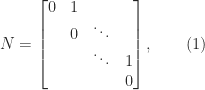
and $N^p = 0$ . The superdiagonal of ones moves up to the right with each increase in the index of the power until it disappears off the top right corner of the matrix.

Matrix $A_4$ has rank $1$ and was constructed using a general formula: if $A = xy^T$ with $y^Tx = 0$ then $A^2 = xy^T xy^T = (y^Tx) xy^T = 0$ . We simply took orthogonal vectors $x =[2, -4, 1]^T$ and $y = [1, 1, 2]^T$ .

If $A$ is nilpotent then every eigenvalue is zero, since $Ax = \lambda x$ with $x\ne 0$ implies $0 = A^nx = \lambda^n x$ or $\lambda = 0$ . Consequently, the trace and determinant of a nilpotent matrix are both zero.

If $A$ is nilpotent and Hermitian or symmetric, or more generally normal ( $A^*A = AA^*$ ), then $A = 0$ , since such a matrix has a spectral decomposition $A = Q \mathrm{diag}(\lambda_i)Q^*$ and the matrix $\mathrm{diag}(\lambda_i)$ is zero. It is only for nonnormal matrices that nilpotency is a nontrivial property, and the best way to understand it is with the Jordan canonical form (JCF). The JCF of a matrix with only zero eigenvalues has the form $A = XJX^{-1}$ , where $J = \mathrm{diag}(J_{m_1},J_{m_2}, \dots, J_{m_p})$ , where $J_{m_i}$ is of the form (1) and hence $J_{m_i}^{m_i} = 0$ . It follows that the index of nilpotency is $k = \max\{\,m_i : i=1\colon p\,\} \le n$ .

What is the rank of an $n\times n$ nilpotent matrix $A$ ? The minimum possible rank is $0$ , attained for the zero matrix. The maximum possible rank is $n-1$ , attained when the JCF of $A$ has just one Jordan block of size $n$ . Any rank between $0$ and $n-1$ is possible: rank $j$ is attained when there is a Jordan block of size $j+1$ and all other blocks are $1\times 1$ .

Finally, while a nilpotent matrix is obviously not invertible, like every matrix it has a Moore–Penrose pseudoinverse. The pseudoinverse of a Jordan block with eigenvalue zero is just the transpose of the block: $N^+ = N^T$ for $N$ in (1).

What Is an Eigenvalue?

An eigenvalue of a square matrix $A$ is a scalar $\lambda$ such that $Ax = \lambda x$ for some nonzero vector $x$ . The vector $x$ is an eigenvector of $A$ and it has the distinction of being a direction that is not changed on multiplication by $A$ .

An $n\times n$ matrix has $n$ eigenvalues. This can be seen by noting that $Ax = \lambda x$ is equivalent to $(\lambda I - A) x = 0$ , which means that $\lambda I - A$ is singular, since $x\ne 0$ . Hence $\det(\lambda I - A) = 0$ . But

$\notag \det(\lambda I - A) = \lambda^n + a_{n-1}\lambda^{n-1} + \cdots + a_1 \lambda + a_0$

is a scalar polynomial of degree $n$ (the characteristic polynomial of $A$ ) with nonzero leading coefficient and so has $n$ roots, which are the eigenvalues of $A$ . Since $\det(\lambda I - A) = \det( (\lambda I - A)^T) = \det(\lambda I - A^T)$ , the eigenvalues of $A^T$ are the same as those of $A$ .

A real matrix may have complex eigenvalues, but they appear in complex conjugate pairs. Indeed $Ax = \lambda x$ implies $\overline{A}\overline{x} = \overline{\lambda} \overline{x}$ , so if $A$ is real then $\overline{\lambda}$ is an eigenvalue of $A$ with eigenvector $\overline{x}$ .

Here are some $2\times 2$ matrices and their eigenvalues.

$\notag \begin{aligned} A_1 &= \begin{bmatrix}1 & 0 \\ 0 & 1 \end{bmatrix}, \quad \lambda = 1,1,\\ A_2 &= \begin{bmatrix}0 & 1 \\ 0 & 0 \end{bmatrix}, \quad \lambda = 0,0,\\ A_3 &= \begin{bmatrix}0 & 1 \\ -1 & 0 \end{bmatrix}, \quad \lambda = \mathrm{i},\mathrm{-i}. \end{aligned}$

Note that $A_1$ and $A_2$ are upper triangular, that is, $a_{ij} = 0$ for $i>j$ . For such a matrix the eigenvalues are the diagonal elements.

A symmetric matrix ( $A^T = A$ ) or Hermitian matrix ( $A^* = A$ , where $A^* = \overline{A}^T$ ) has real eigenvalues. A proof is $Ax = \lambda x \Rightarrow x^*A^* = \overline{\lambda} x^*$ so premultiplying the first equation by $x^*$ and postmultiplying the second by $x$ gives $x^*Ax = \lambda x^*x$ and $x^*Ax = \overline{\lambda} x^*x$ , which means that $(\lambda-\overline{\lambda})x^*x = 0$ , or $\lambda=\overline{\lambda}$ since $x^*x \ne 0$ . The matrix $A_1$ above is symmetric.

A skew-symmetric matrix ( $A^T = -A$ ) or skew-Hermitian complex matrix ( $A^* = -A$ ) has pure imaginary eigenvalues. A proof is similar to the Hermitian case: $Ax = \lambda x \Rightarrow -x^*A = x^*A^* = \overline{\lambda} x^*$ and so $x^*Ax$ is equal to both $\lambda x^*x$ and $-\overline{\lambda} x^*x$ , so $\lambda = -\overline{\lambda}$ . The matrix $A_3$ above is skew-symmetric.

In general, the eigenvalues of a matrix $A$ can lie anywhere in the complex plane, subject to restrictions based on matrix structure such as symmetry or skew-symmetry, but they are restricted to the disc centered at the origin with radius $\|A\|$ , because for any matrix norm $\|\cdot\|$ it can be shown that every eigenvalue satisfies $|\lambda| \le \|A\|$ .

Here are some example eigenvalue distributions, computed in MATLAB. (The eigenvalues are computed at high precision using the Advanpix Multiprecision Computing Toolbox in order to ensure that rounding errors do not affect the plots.) The second and third matrices are real, so the eigenvalues are symmetrically distributed about the real axis. (The first matrix is complex.)

Although this article is about eigenvalues we need to say a little more about eigenvectors. An $n\times n$ matrix $A$ with distinct eigenvalues has $n$ linearly independent eigenvectors. Indeed it is diagonalizable: $A = XDX^{-1}$ for some nonsingular matrix $X$ with $D = \mathrm{diag}(\lambda_i)$ the matrix of eigenvalues. If we write $X$ in terms of its columns as $X = [x_1,x_2,\dots,x_n]$ then $AX = XD$ is equivalent to $Ax_i = \lambda _i x_i$ , $i=1\colon n$ , so the $x_i$ are eigenvectors of $A$ . The matrices $A_1$ and $A_3$ above both have two linearly independent eigenvectors.

If there are repeated eigenvalues there can be less than $n$ linearly independent eigenvectors. The matrix $A_2$ above has only one eigenvector: the vector $\left[\begin{smallmatrix}1 \\ 0 \end{smallmatrix}\right]$ (or any nonzero scalar multiple of it). This matrix is a Jordan block. The matrix $A_1$ shows that a matrix with repeated eigenvalues can have linearly independent eigenvectors.

Here are some questions about eigenvalues.

What matrix decompositions reveal eigenvalues? The answer is the Jordan canonical form and the Schur decomposition. The Jordan canonical form shows how many linearly independent eigenvectors are associated with each eigenvalue.
Can we obtain better bounds on where eigenvalues lie in the complex plane? Many results are available, of which the most well-known is Gershgorin’s theorem.
How can we compute eigenvalues? Various methods are available. The QR algorithm is widely used and is applicable to all types of eigenvalue problems.

Finally, we note that the concept of eigenvalue is more general than just for matrices: it extends to nonlinear operators on finite or infinite dimensional spaces.

References

Many books include treatments of eigenvalues of matrices. We give just three examples.

Gene Golub and Charles F. Van Loan, Matrix Computations, fourth edition, Johns Hopkins University Press, Baltimore, MD, USA, 2013.
Roger A. Horn and Charles R. Johnson, Matrix Analysis, second edition, Cambridge University Press, 2013. My review of the second edition.
Carl D. Meyer, Matrix Analysis and Applied Linear Algebra, Society for Industrial and Applied Mathematics, Philadelphia, PA, USA, 2000.

Month: November 2022

What Is Gershgorin’s Theorem?

Notes

References

Related Blog Posts

What Is a Nilpotent Matrix?

Related Blog Posts

What Is an Eigenvalue?

References

Related Blog Posts

Notes

References

Related Blog Posts

Share this:

Related Blog Posts

Share this:

References

Related Blog Posts

Share this: