What Is Rounding?

Rounding is the transformation of a number expressed in a particular base to a number with fewer digits. For example, in base 10 we might round the number $x = 7.146$ to $7.15$ , which can be described as rounding to three significant digits or two decimal places. Rounding does not change a number if it already has the requisite number of digits.

The three main uses of rounding are

to simplify a number in base 10 for human consumption,
to represent a constant such as $1/3$ , $\pi$ , or $\sqrt{7}$ in floating-point arithmetic,
to convert the result of an elementary operation (an addition, multiplication, or division) on floating-point numbers back into a floating-point number.

The floating-point numbers may be those used on a computer (base 2) or a pocket calculator (base 10).

Rounding can be done in several ways.

Round to Nearest

The most common form of rounding is to round to the nearest number with the specified number of significant digits or decimal places. In the example above, the two nearest numbers to $x$ with three significant digits are $7.14$ and $7.15$ , at distances $0.006$ and $0.004$ , respectively, from $x$ . The nearest of these two numbers, $7.15$ , is chosen.

What happens if the two candidate numbers are equally close? We need a rule for breaking the tie. The most common choices are

round to even: choose the number with an even last digit,
round to odd: choose the number with an odd last digit.

If we round $1.85$ to two significant digits, the result is $1.8$ with round to even and $1.9$ with round to odd.

There are several reasons for preferring to break ties with round to even.

In bases 2 and 10 a subsequent rounding to one less place does not involve a tie. Thus we have the rounding sequence $2.445$ , $2.44$ , $2.4$ , $2$ with round to even, but $2.445$ , $2.45$ , $2.5$ , $3$ with round to odd.
For base 2, round to even results in integers more often, as a consequence of producing a zero least significant bit.
In base 10, after round to even a rounded number can be halved without error.

IEEE Standard 745 for floating-point arithmetic supports three tie-breaking methods: round to even (the default), round to the number with larger magnitude, and round towards zero (introduced in the 2019 revision for use with the standard’s new augmented operations).

The tie-breaking rule taught in UK schools, for decimal arithmetic, is to round up on ties. The rounding rule then becomes: round down if the first digit to be dropped is $4$ or less and otherwise round up.

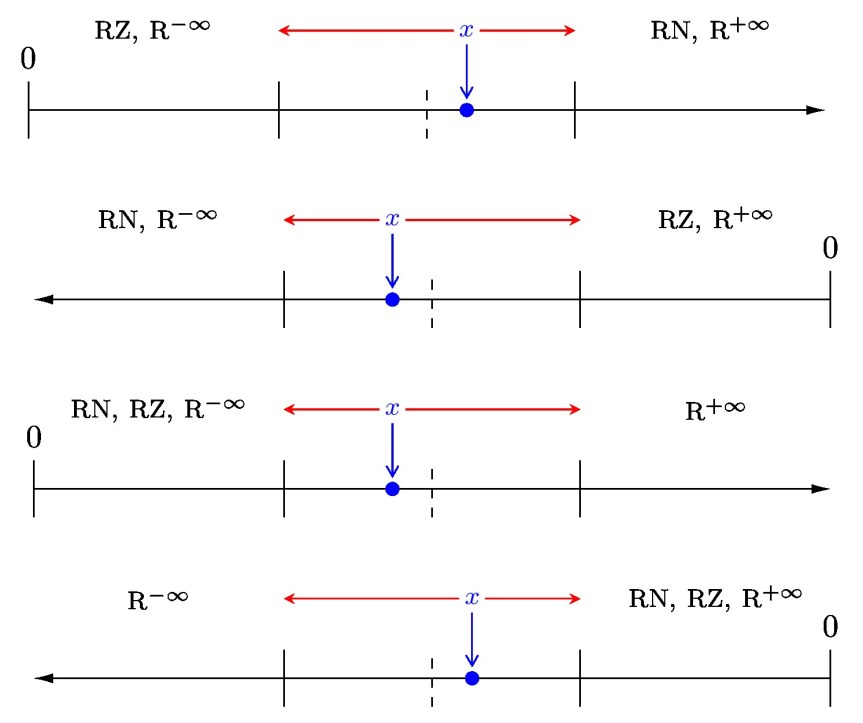
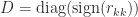
Round Towards Plus or Minus Infinity

Another possibility is to round to the next larger number with the specified number of digits, which is known as round towards plus infinity (or round up). Then $1.85$ rounds to $1.9$ and $-2.34$ rounds to $-2.3$ . Similarly, with round towards minus infinity (or round down) we round to the next smaller number, so that $1.85$ rounds to $1.8$ and $-2.34$ rounds to $-2.4$ .

This form of rounding is used in interval arithmetic, where an interval guaranteed to contain the exact result is computed in floating-point arithmetic.

Round Towards Zero

In this form of rounding we round towards zero, that is, we round $x$ down if $x > 0$ and round it up if $x < 0$ . This is also known as chopping, or truncation.

Stochastic Rounding

Stochastic rounding was proposed in the 1950s and is attracting renewed interest, especially in machine learning. It rounds up or down randomly. It come in two forms. The first form rounds up or down with equal probability $1/2$ . To describe the second form, let $x$ be the given number and let $x_1 x$ be the candidates for the result of rounding. We round up to $x_2$ with probability $(x-x_1)/(x_2-x_1)$ and down to $x_1$ with probability $(x_2-x)/(x_2-x_1)$ ; note that these probabilities sum to $1$ . In floating-point arithmetic, stochastic rounding overcomes the problem that can arise in summing a set of numbers whereby some individual summands are so small that they do not contribute to the computed sum even though they contribute to the exact sum.

The diagrams below illustrate round to nearest (RN), round towards zero (RZ), round towards plus infinity ( $\mathrm{R}^{+\infty}$ ), and round towards minus infinity ( $\mathrm{R}^{-\infty}$ ). They show the number $x$ to be rounded in four different configurations with respect to the origin and the midpoint (drawn with a dotted line) of the interval between the two candidate rounding results (drawn with a solid line). The red arrows point to the two possible results of rounding.

Real World Rounding

The European Commission’s rules for converting currencies of Member States into Euros (from the time of the creation of the Euro) specify that “half-way results are rounded up” (rounded to plus infinity). (PDF link)

The International Association of Athletics Federations (IAAF) specifies in Rule 165 of its Competition Rules 2018–2019 that all times of track races up to 10,000m should be recorded to a precision of 0.01 second, with rounding to plus infinity. In 2006, the athlete Justin Gatlin was wrongly credited with breaking the 100m world record when his official time of 9.766 seconds was rounded down to 9.76 seconds. Under the IAAF rules it should have been rounded up to 9.77 seconds, matching the world record set by Asafa Powell the year before. The error was discovered several days after the race.

In meteorology, rounding to nearest with ties broken by rounding to odd is favoured. Hunt suggests that the reason is to avoid falsely indicating that it is freezing. Thus $0.5^\circ$ C and $32.5^\circ$ F round to $1^\circ$ C and $33^\circ$ F instead of $0^\circ$ C and $32^\circ$ F.

Useful Tool

The $\LaTeX$ package siunitx has the ability to round numbers (in base 10) to a specified number of decimal places or significant figures.

References

This is a minimal set of references, which contain further useful references within.

Michael P. Connolly, Nicholas J. Higham, and Theo Mary, Stochastic Rounding and Its Probabilistic Backward Error Analysis, MIMS EPrint 2020.12, Manchester Institute for Mathematical Sciences, The University of Manchester, UK, April 2020.
Nicholas J. Higham, Accuracy and Stability of Numerical Algorithms, second edition, Society for Industrial and Applied Mathematics, Philadelphia, PA, USA, 2002.
Julian Hunt, Rounding and Other Approximations for Measurements, Records and Targets, Mathematics Today 33, 73–77, 1997.
IEEE Standard for Floating-Point Arithmetic, IEEE Std 754-2019 (Revision of IEEE 754-2008), IEEE Computer Society, New York, 2019.

What Is a Random Orthogonal Matrix?

Various explicit parametrized formulas are available for constructing orthogonal matrices. To construct a random orthogonal matrix we can take such a formula and assign random values to the parameters. For example, a Householder matrix $H = I - 2uu^T/(u^Tu)$ is orthogonal and symmetric and we can choose the nonzero vector $u$ randomly. Such an example is rather special, though, as it is a rank- $1$ perturbation of the identity matrix.

What is usually meant by a random orthogonal matrix is a matrix distributed according to the Haar measure over the group of orthogonal matrices. The Haar measure provides a uniform distribution over the orthogonal matrices. Indeed it is invariant under multiplication on the left and the right by orthogonal matrices: if $Q$ is from the Haar distribution then so is $UQV$ for any orthogonal (possibly non-random) $U$ and $V$ . A random Householder matrix is not Haar distributed.

A matrix from the Haar distribution can be generated as the orthogonal factor in the QR factorization of a random matrix with elements from the standard normal distribution (mean $0$ , variance $1$ ). In MATLAB this is done by the code

[Q,R] = qr(randn(n));
Q = Q*diag(sign(diag(R)));

The statement [Q,R] = qr(randn(n)), which returns the orthogonal factor $Q$ , is not enough on its own to give a Haar distributed matrix, because the QR factorization is not unique. The second line adjusts the signs so that $Q$ is from the unique factorization in which the triangular factor $R$ has nonnegative diagonal elements. This construction requires $2n^3$ flops.

A more efficient construction is possible, as suggested by Stewart (1980). Let $x_k$ be an $(n-k+1)$ -vector of elements from the standard normal distribution and let $H_k$ be the Householder matrix that reduces $x_k$ to $r_{kk}e_1$ , where $e_1$ is the first unit vector. Then 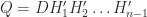$Q = DH'_1H'_2\dots H'_{n-1}$ is Haar distributed, where $H'_k = \mathrm{diag}(I_{k-1}, H_k)$ , $D = \mathrm{diag}(\mathrm{sign}(r_{kk}))$ , and $r_{nn} = x_n$ . This construction expresses $Q$ as the product of $n-1$ Householder matrices of growing effective dimension, and the product can be formed from right to left in $4n^3/3$ flops. The MATLAB statement Q = gallery('qmult',n) carries out this construction.

A similar construction can be made using Givens rotations (Anderson et al., 1987).

Orthogonal matrices from the Haar distribution can also be formed as $Q = A (A^TA)^{-1/2}$ , where the elements of $A$ are from the standard normal distribution. This $Q$ is the orthogonal factor in the polar decomposition $A = QH$ (where $H$ is symmetric positive semidefinite).

Random orthogonal matrices arise in a variety of applications, including Monte Carlo simulation, random matrix theory, machine learning, and the construction of test matrices with known eigenvalues or singular values.

All these ideas extend to random unitary (complex) matrices. In MATLAB, Haar distributed unitary matrices can be constructed by the code

[Q,R] = qr(complex(randn(n),randn(n)));
Q = Q*diag(sign(diag(R)));

This code exploits the fact that the $R$ factor computed by MATLAB has real diagonal entries. If the diagonal of $R$ were complex then this code would need to be modified to use the complex sign function given by $\mathrm{sign}(z) = z/|z|$ .

References

This is a minimal set of references, which contain further useful references within.

T. W. Anderson, I. Olkin and L. G. Underhill, Generation of random orthogonal matrices, SIAM J. Sci. Statist. Comput. 8(4), 625–629, 1987.
Alan Edelman and N. Raj Rao, Random matrix theory, Acta Numerica, 14, 233–297, 2005.
Nicholas J. Higham, Accuracy and Stability of Numerical Algorithms, second edition, Society for Industrial and Applied Mathematics, Philadelphia, PA, USA, 2002. (Chapter 28.)
Francesco Mezzadri, How to generate random matrices from the classical compact groups, Notices Amer. Math. Soc. 54(5), 592–604, 2007
G. W. Stewart, The efficient generation of random orthogonal matrices with an application to condition estimators, SIAM J. Numer. Anal. 17(3), 403–409, 1980.

What Is a Correlation Matrix?

In linear algebra terms, a correlation matrix is a symmetric positive semidefinite matrix with unit diagonal. In other words, it is a symmetric matrix with ones on the diagonal whose eigenvalues are all nonnegative.

The term comes from statistics. If $x_1, x_2, \dots, x_n$ are column vectors with $m$ elements, each vector containing samples of a random variable, then the corresponding $n\times n$ covariance matrix $V$ has $(i,j)$ element

$v_{ij} = \mathrm{cov}(x_i,x_j) = \displaystyle\frac{1}{n-1} (x_i - \overline{x}_i)^T (x_j - \overline{x}_j),$

where $\overline{x}_i$ is the mean of the elements in $x_i$ . If $v$ has nonzero diagonal elements then we can scale the diagonal to 1 to obtain the corresponding correlation matrix

$C = D^{-1/2} V D^{-1/2},$

where $D = \mathrm{diag}(v_{ii})$ . The $(i,j)$ element $c_{ij} = v_{ii}^{-1/2} v_{ij} v_{jj}^{-1/2}$ is the correlation between the variables $x_i$ and $x_j$ .

Here are a few facts.

The elements of a correlation matrix lie on the interval $[-1, 1]$ .
The eigenvalues of a correlation matrix lie on the interval $[0,n]$ .
The eigenvalues of a correlation matrix sum to $n$ (since the eigenvalues of a matrix sum to its trace).
The maximal possible determinant of a correlation matrix is $1$ .

It is usually not easy to tell whether a given matrix is a correlation matrix. For example, the matrix

$A = \begin{bmatrix} 1 & 1 & 0\\ 1 & 1 & 1\\ 0 & 1 & 1 \end{bmatrix}$

is not a correlation matrix: it has eigenvalues $-0.4142$ , $1.0000$ , $2.4142$ . The only value of $a_{13}$ and $a_{31}$ that makes $A$ a correlation matrix is $1$ .

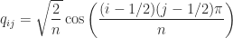
A particularly simple class of correlation matrices is the one-parameter class $A_n$ with every off-diagonal element equal to $w$ , illustrated for $n = 3$ by

$A_3 = \begin{bmatrix} 1 & w & w\\ w & 1 & w\\ w & w & 1 \end{bmatrix}.$

The matrix $A_n$ is a correlation matrix for $-1/(n-1) \le w \le 1$ .

In some applications it is required to generate random correlation matrices, for example in Monte-Carlo simulations in finance. A method for generating random correlation matrices with a specified eigenvalue distribution was proposed by Bendel and Mickey (1978); Davies and Higham (2000) give improvements to the method. This method is implemented in the MATLAB function gallery('randcorr').

Obtaining or estimating correlations can be difficult in practice. In finance, market data is often missing or stale; different assets may be sampled at different time points (e.g., some daily and others weekly); and the matrices may be generated from different parametrized models that are not consistent. Similar problems arise in many other applications. As a result, correlation matrices obtained in practice may not be positive semidefinite, which can lead to undesirable consequences such as an investment portfolio with negative risk.

In risk management and insurance, matrix entries may be estimated, prescribed by regulations or assigned by expert judgement, but some entries may be unknown.

Two problems therefore commonly arise in connection with correlation matrices.

Nearest Correlation Matrix

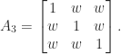
Here, we have an approximate correlation matrix $A$ that has some negative eigenvalues and we wish to replace it by the nearest correlation matrix. The natural choice of norm is the Frobenius norm, $\|A\|_F = \bigl(\sum_{i,j} a_{ij}^2\bigr)^{1/2}$ , so we solve the problem

$\min \{ \, \|A-C\|_F: C~\textrm{is a correlation matrix} \,\}.$

We may also have a requirement that certain elements of $C$ remain fixed. And we may want to weight some elements more than others, by using a weighted Frobenius norm. These are convex optimization problems and have a unique solution that can be computed using the alternating projections method (Higham, 2002) or a Newton algorithm (Qi and Sun, 2006; Borsdorf and Higham, 2010).

Another variation requires $C$ to have factor structure, which means that the off-diagonal agrees with that of a rank- $k$ matrix for some given $k$ (Borsdorf, Higham, and Raydan, 2010). Yet another variation imposes a constraint that $C$ has a certain rank or a rank no larger than a certain value. These problems are non-convex, because of the objective function and the rank constraint, respectively.

Another approach that can be used for restoring definiteness, although it does not in general produce the nearest correlation matrix, is shrinking, which constructs a convex linear combination $A = \alpha C + (1-\alpha)M$ , where $M$ is a target correlation matrix (Higham, Strabić, and Šego, 2016). Shrinking can readily incorporate fixed blocks and weighting.

Correlation Matrix Completion

Here, we have a partially specified matrix and we wish to complete it, that is, fill in the missing elements in order to obtain a correlation matrix. It is known that a completion is possible for any set of specified entries if the associate graph is chordal (Grone et al., 1994). In general, if there is one completion there are many, but there is a unique one of maximal determinant, which is elegantly characterized by the property that the inverse contains zeros in the positions of the unspecified entries.

References

This is a minimal set of references, and they cite further useful references.

Rüdiger Borsdorf, Nicholas J. Higham and Marcos Raydan, Computing a nearest correlation matrix with factor structure, SIAM J. Matrix Anal. Appl. 31(5), 2603–2622, 2010
Rüdiger Borsdorf and Nicholas J. Higham, A preconditioned Newton algorithm for the nearest correlation matrix, J. Numer. Anal. 30(1), 94–107, 2010.
Philip I. Davies and Nicholas J. Higham, Numerically stable generation of correlation matrices and their factors, BIT 40(4), 640–651, 2000
Dan I. Georgescu, Nicholas J. Higham and Gareth W. Peters, Explicit solutions to correlation matrix completion problems, with an application to risk management and insurance, Roy. Soc. Open Sci. 5(3), 1–11, 2018.
Robert Grone, Charles R. Johnson, Eduardo M. Sá and Henry Wolkowicz, Positive definite completions of partial Hermitian matrices, Linear Algebra Appl. 58, 109–124, 1984.
Nicholas J. Higham, Computing the nearest correlation matrix—A problem from finance, IMAJNA J. Numer. Anal. 22(3), 329–343, 2002.
Houduo Qi and Defeng Sun, A quadratically convergent Newton method for computing the nearest correlation matrix, SIAM J. Matrix Anal. Appl. 28(2), 360–385, 2006
Nicholas J. Higham, Nataša Strabić and Vedran Šego, Restoring definiteness via shrinking, with an application to correlation matrices with a fixed block, SIAM Rev. 58(2), 245–263, 2016.
Numerical Algorithms Group, Nearest Correlation Matrix, 2019.

What Is a Hadamard Matrix?

A Hadamard matrix is an $n\times n$ matrix with elements $\pm 1$ and mutually orthogonal columns. For example,

$\left[\begin{array}{rrrr} 1 & 1 & 1 & 1\\ 1 & -1 & 1 & -1\\ 1 & 1 & -1 & -1\\ 1 & -1 & -1 & 1 \end{array}\right]$

is a Hadamard matrix.

A necessary condition for an $n\times n$ Hadamard matrix to exist with $n > 2$ is that $n$ is divisible by $4$ , but it is not known if a Hadamard matrix exists for every such $n$ .

A Hadamard matrix of order 428 was found for the first time in 2005. The smallest multiple of $4$ for which a Hadamard matrix has not been found is 668.

A Hadamard matrix satisfies $H^T H = nI$ , so $H^{-1} = n^{-1}H^T$ . It also follows that $\det(H) = \pm n^{n/2}$ . Hadamard’s inequality states that for an $n\times n$ real matrix $A$ , $|\det(A)| \le \prod_{k=1}^n \|a_k\|_2$ , where $a_k$ is the $k$ th column of $A$ . A Hadamard matrix achieves equality in this inequality (as does any matrix with orthogonal columns).

Hadamard matrices can be generated with a recursive (Kronecker product) construction: if $H$ is a Hadamard matrix then so is

$\left[\begin{array}{rr} H & H\\ H & -H \end{array}\right].$

So starting with a Hadamard matrix of size $m$ , one can build up matrices of size $2^km$ for $k = 1,2,\dots$ . The MATLAB hadamard function uses this technique. It includes the following Hadamard matrix of order 12, for which we simply display the signs of the elements:

$\left[\begin{array}{rrrrrrrrrrrr} {}+ & + & + & + & + & 1 & + & + & + & + & + & +\\ {}+ & - & + & - & + & + & + & - & - & - & + & -\\ {}+ & - & - & + & - & + & + & + & - & - & - & +\\ {}+ & + & - & - & + & - & + & + & + & - & - & -\\ {}+ & - & + & - & - & + & - & + & + & + & - & -\\ {}+ & - & - & + & - & - & + & - & + & + & + & -\\ {}+ & - & - & - & + & - & - & + & - & + & + & +\\ {}+ & + & - & - & - & + & - & - & + & - & + & +\\ {}+ & + & + & - & - & - & + & - & - & + & - & +\\ {}+ & + & + & + & - & - & - & + & - & - & + & -\\ {}+ & - & + & + & + & - & - & - & + & - & - & +\\ {}+ & + & - & + & + & + & - & - & - & + & - & - \end{array}\right].$

Hadamard matrices have applications in optimal design theory, coding theory, and graph theory.

In numerical analysis, Hadamard matrices are of interest because when LU factorization is performed on them they produce a growth factor of at least $n$ , for any form of pivoting. Evidence suggests that the growth factor for complete pivoting is exactly $n$ , but this has not been proved. It has been proved that any $n\times n$ Hadamard matrix has growth factor $n$ for complete pivoting for $n = 12$ and $n = 16$ .

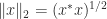
An interesting property of Hadamard matrices is that the $p$ -norm (the matrix norm subordinate to the vector $p$ -norm) is known explicitly for all $p$ :

$\|H\|_p = \max\bigl( n^{1/p}, n^{1-1/p} \bigr), \quad 1\le p\le \infty.$

References

This is a minimal set of references, which contain further useful references within.

A. Hedayat and W. D. Wallis, Hadamard Matrices and Their Applications, Ann. Statist. 6, 1184–1238, 1978.
Nicholas J. Higham, Accuracy and Stability of Numerical Algorithms, second edition, Society for Industrial and Applied Mathematics, Philadelphia, PA, USA, 2002.
Christos D. Kravvaritis, Hadamard Matrices: Insights into Their Growth Factor and Determinant Computations, in M. Themistocles Rassias and Vijay Gupta, eds, Mathematical Analysis, Approximation Theory and Their Applications, Springer-Verlag, Berlin, 383–415, 2016.
Christos Kravvaritis and Marilena Mitrouli, The Growth Factor of a Hadamard Matrix of Order $16$ is $16$ , Numer. Linear Algebra Appl. 16, 715–743, 2009.
H. Kharaghani and B. Tayfeh-Rezaie, A Hadamard Matrix of Order $428$ , J. Combin. Des. 56, 435–440, 2005.
A Library of Hadamard Matrices, N. J. A. Sloane.

What Is an Orthogonal Matrix?

A real, square matrix $Q$ is orthogonal if $Q^TQ = QQ^T = I$ (the identity matrix). Equivalently, $Q^{-1} = Q^T$ . The columns of an orthogonal matrix are orthonormal, that is, they have 2-norm (Euclidean length) $1$ and are mutually orthogonal. The same is true of the rows.

Important examples of orthogonal matrices are rotations and reflectors. A $2\times 2$ rotation matrix has the form

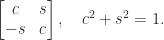
$\begin{bmatrix} c & s \\ -s& c \\ \end{bmatrix}, \quad c^2 + s^2 = 1.$

For such a matrix, $c = \cos \theta$ and $s = \sin \theta$ for some $\theta$ , and the multiplication $y = Qx$ for a $2\times 1$ vector $x$ represents a rotation through an angle $\theta$ radians. An $n\times n$ rotation matrix is formed by embedding the $2\times 2$ matrix into the identity matrix of order $n$ .

A Householder reflector is a matrix of the form $H = I - 2uu^T/(u^Tu)$ , where $u$ is a nonzero $n$ -vector. It is orthogonal and symmetric. When applied to a vector it reflects the vector about the hyperplane orthogonal to $v$ . For $n = 2$ , such a matrix has the form

$\begin{bmatrix} c & s \\ s& -c \\ \end{bmatrix}, \quad c^2 + s^2 = 1.$

Here is the $4\times 4$ Householder reflector corresponding to $v = [1,1,1,1]^T/2$ :

$\frac{1}{2} \left[\begin{array}{@{\mskip2mu}rrrr@{\mskip2mu}} 1 & -1 & -1 & -1\\ -1 & 1 & -1 & -1\\ -1 & -1 & 1 & -1\\ -1 & -1 & -1 & 1\\ \end{array}\right].$

This is $1/2$ times a Hadamard matrix.

Various explicit formulas are known for orthogonal matrices. For example, the $n\times n$ matrices with $(i,j)$ elements

$q_{ij} = \displaystyle\frac{2}{\sqrt{2n+1}} \sin \left(\displaystyle\frac{2ij\pi}{2n+1}\right)$

and

$q_{ij} = \sqrt{\displaystyle\frac{2}{n}}\cos \left(\displaystyle\frac{(i-1/2)(j-1/2)\pi}{n} \right)$

are orthogonal. These and other orthogonal matrices, as well as diagonal scalings of orthogonal matrices, are constructed by the MATLAB function gallery('orthog',...).

Here are some properties of orthogonal matrices.

All the eigenvalues are on the unit circle, that is, they have modulus $1$ .
All the singular values are $1$ .
The $2$ -norm condition number is $1$ , so orthogonal matrices are perfectly conditioned.
Multiplication by an orthogonal matrix preserves Euclidean length: $\|Qx\|_2 = \|x\|_2$ for any vector $x$ .
The determinant of an orthogonal matrix is $\pm 1$ . A rotation has determinant $1$ while a reflection has determinant $-1$ .

Orthogonal matrices can be generated from skew-symmetric ones. If $S$ is skew-symmetric ( $S = -S^T$ ) then $\exp(S)$ (the matrix exponential) is orthogonal and the Cayley transform $(I-S)(I+S)^{-1}$ is orthogonal as long as $S$ has no eigenvalue equal to $-1$ .

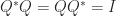Unitary matrices are complex square matrices $Q$ for which $Q^*Q = QQ^* = I$ , where $Q^*$ is the conjugate transpose of $Q$ . They have analogous properties to orthogonal matrices.

What Is a Generalized Inverse of a Matrix?

The matrix inverse is defined only for square nonsingular matrices. A generalized inverse is an extension of the concept of inverse that applies to square singular matrices and rectangular matrices. There are many definitions of generalized inverses, all of which reduce to the usual inverse when the matrix is square and nonsingular.

A large class of generalized inverses of an $m \times n$ matrix $A$ can be defined in terms of the Moore–Penrose conditions, in which $X$ is $n\times m$ :

$\begin{array}{rcrc} \mathrm{(1)} & AXA = A, \; & \mathrm{(2)} & XAX=X,\\ \mathrm{(3)} & (AX)^* = AX, \; & \mathrm{(4)} & (XA)^* = XA. \end{array}$

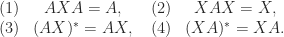
Here, the superscript $*$ denotes the conjugate transpose. A 1-inverse is any $X$ satisfying condition (1), a (1,3)-inverse is any $X$ satisfying conditions (1) and (3), and so on for any subset of the four conditions.

Condition (1) implies that if $Ax = b$ then $A(Xb) = A (XAx) = AXAx = Ax = b$ , so $Xb$ solves the equation, meaning that any 1-inverse is an equation-solving inverse. Condition (2) implies that $X = 0$ if $A = 0$ .

A (1,3) inverse can be shown to provide a least squares solution to an inconsistent linear system. A (1,4) inverse can be shown to provide the minimum 2-norm solution of a consistent linear system (where the 2-norm is defined by $\|x\|_2 = (x^*x)^{1/2}$ ).

There is not a unique matrix satisfying any one, two, or three of the Moore–Penrose conditions. But there is a unique matrix satisfying all four of the conditions, and it is called the Moore-Penrose pseudoinverse, denoted by $A^+$ or $A^{\dagger}$ . For any system of linear equations $Ax = b$ , $x = A^+b$ minimizes $\|Ax - b\|_2$ and has the minimum 2–norm over all minimizers.

The pseudoinverse can be expressed in terms of the singular value decomposition (SVD). If $A = U\Sigma V^*$ is an SVD, where the $m\times m$ matrix $U$ and $n\times n$ matrix $V$ are orthogonal, and $\Sigma = \mathrm{diag}(\sigma_1,\dots , \sigma_n)$ with $\sigma_1 \ge \sigma_2 \ge \cdots \ge \sigma_r > \sigma_{r+1} = \cdots =\sigma_n = 0$ (so that $\mathrm{rank}(A) = r$ ), then

$A^+ = V\mathrm{diag}(\sigma_1^{-1},\dots,\sigma_r^{-1},0,\dots,0)U^*.$

In MATLAB, the function pinv computes $A^+$ using this formula. If $\mathrm{rank}(A) = n$ then the concise formula $A^+ = (A^*A)^{-1}A^*$ holds.

For square matrices, the Drazin inverse is the unique matrix $A^D$ such that

$A^D A A^D = A^D, \quad A A ^D = A^D A, \quad A^{k+1} A^D = A^k,$

where $k = \mathrm{index}(A)$ . The first condition is the same as the second of the Moore–Penrose conditions, but the second and third have a different flavour. The index of a matrix of $A$ is the smallest nonnegative integer $k$ such that $\mathrm{rank}(A^k) = \mathrm{rank}(A^{k+1})$ ; it is characterized as the dimension of the largest Jordan block of $A$ with eigenvalue zero.

If $\mathrm{index}(A)=1$ then $A^D$ is also known as the group inverse of $A$ and is denoted by $A^\#$ . The Drazin inverse is an equation-solving inverse precisely when $\mathrm{index}(A)\le 1$ , for then $AA^DA=A$ , which is the first of the Moore–Penrose conditions.

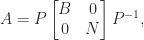
The Drazin inverse can be represented explicitly as follows. If

$A = P \begin{bmatrix} B & 0 \\ 0 & N \end{bmatrix} P^{-1},$

where $P$ and $B$ are nonsingular and $N$ has only zero eigenvalues, then

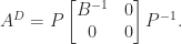
$A^D = P \begin{bmatrix} B^{-1} & 0 \\ 0 & 0 \end{bmatrix} P^{-1}.$

Here is the pseudoinverse and the Drazin inverse for a particular matrix with index $2$ :

$A = \left[\begin{array}{rrr} 1 & -1 & -1\\[3pt] 0 & 0 & -1\\[3pt] 0 & 0 & 0 \end{array}\right], \quad A^+ = \left[\begin{array}{rrr} \frac{1}{2} & -\frac{1}{2} & 0\\[3pt] -\frac{1}{2} & \frac{1}{2} & 0\\[3pt] 0 & -1 & 0 \end{array}\right], \quad A^D = \left[\begin{array}{rrr} 1 & -1 & 0\\[3pt] 0 & 0 & 0\\[3pt] 0 & 0 & 0 \end{array}\right].$

Applications

The Moore–Penrose pseudoinverse is intimately connected with orthogonality, whereas the Drazin inverse has spectral properties related to those of the original matrix. The pseudoinverse occurs in all kinds of least squares problems. Applications of the Drazin inverse include population modelling, Markov chains, and singular systems of linear differential equations. It is not usually necessary to compute generalized inverses, but they are valuable theoretical tools.

References

This is a minimal set of references, which contain further useful references within.

Adi Ben-Israel, The Moore of the Moore–Penrose Inverse, Electron. J. Linear Algebra 9, 150–157, 2002.
Adi Ben-Israel and Thomas N. E. Greville, Generalized Inverses: Theory and Applications, second edition, Springer-Verlag, New York, 2003
Stephen Campbell and Carl Meyer, Generalized Inverses of Linear Transformations, Society for Industrial and Applied Mathematics, Philadelphia, PA, USA, 2009. published (Originally published by Pitman in 1979.)
Stephen J. Kirkland and Michael Neumann, Group Inverses and $M$ -Matrices and their Applications, Chapman and Hall/CRC, 2013
Guorong Wang, Yimin Wei and Sanzheng Qiao, Generalized Inverses: Theory and Computations, second edition, Springer-Verlag, Singapore, 2018.

Month: April 2020

What Is Rounding?

Round to Nearest

Round Towards Plus or Minus Infinity

Round Towards Zero

Stochastic Rounding

Real World Rounding

Useful Tool

References

Related Blog Posts

What Is a Random Orthogonal Matrix?

References

Related Blog Posts

What Is a Correlation Matrix?

Nearest Correlation Matrix

Correlation Matrix Completion

References

Related Blog Posts

What Is a Hadamard Matrix?

References

Related Blog Posts

What Is an Orthogonal Matrix?

Related Blog Posts

What Is a Generalized Inverse of a Matrix?

Applications

References

Related Blog Posts

Round to Nearest

Round Towards Plus or Minus Infinity

Round Towards Zero

Stochastic Rounding

Real World Rounding

Useful Tool

References

Related Blog Posts

Share this:

References

Related Blog Posts

Share this:

Nearest Correlation Matrix

Correlation Matrix Completion

References

Related Blog Posts

Share this:

References

Related Blog Posts

Share this:

Related Blog Posts

Share this:

Applications

References

Related Blog Posts

Share this: