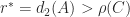
Given a symmetric matrix and a nonnegative number 
Distance can be measured in any norm, but the most common choice is the Frobenius norm, 
This problem occurs in a very wide range of applications. A typical scenario is that a covariance matrix is approximated in some way that does not guarantee positive semidefinitess, for example by treating blocks of the matrix independently. In machine learning, some methods use indefinite kernels and these can require an indefinite similarity matrix to be replaced by a semidefinite one. When 
The following theorem gives the solution to the problem for the Frobenius norm.
Theorem (Cheng and Higham, 1998).
Let the symmetric matrix
have the spectral decomposition
and let
. The unique matrix with smallest eigenvalue at least
in the Frobenius norm is given by

The theorem says that there is a unique nearest matrix and that is has the same eigenvectors as 


One can pose the same nearness problem for nonsymmetric 

For the 


Theorem (Halmos, 1972).
The
where
and a nearest matrix is


When 

Clearly, 


The Frobenius norm solution 

Halmos’s theorem simplifies the computation of 


Example
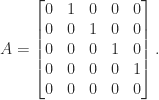
For a numerical example (in MATLAB), we take the Jordan block
The symmetric part of 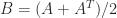
>> A = gallery('jordbloc',5,0); As = sym(A); eig_B = eig((As+As')/2)'
eig_B =
[-1/2, 0, 1/2, -3^(1/2)/2, 3^(1/2)/2]
>> double(eig_B)
ans =
  -5.0000e-01            0   5.0000e-01  -8.6603e-01   8.6603e-01
The nearest symmetric positive semidefinite matrix to
B = (A + A')/2; [Q,D] = eig(B); d = diag(D); X_F = Q*diag(max(d,0))*Q';
We can improve this code by using the implicit expansion feature of MATLAB to avoid forming a diagonal matrix. Since the computed result is not exactly symmetric because of rounding errors, we also need to replace it by the nearest symmetric matrix:
[Q,d] = eig(B,'vector'); X_F = Q*(max(d,0).*Q'); X_F = (X_F + X_F')/2;
We obtain
X_F =
 1.972e-01   2.500e-01   1.443e-01  -4.163e-17  -5.283e-02
 2.500e-01   3.415e-01   2.500e-01   9.151e-02  -1.665e-16
 1.443e-01   2.500e-01   2.887e-01   2.500e-01   1.443e-01
-4.163e-17   9.151e-02   2.500e-01   3.415e-01   2.500e-01
-5.283e-02  -1.665e-16   1.443e-01   2.500e-01   1.972e-01
which has eigenvalues
-3.517e-17 7.246e-17 9.519e-17 5.000e-01 8.660e-01
Notice that the three eigenvalues that would be zero in exact arithmetic are of order the unit roundoff. A nearest matrix in the
X_2 =
 8.336e-01   5.000e-01   1.711e-01   0.000e+00  -1.756e-02
 5.000e-01   6.625e-01   5.000e-01   1.887e-01   0.000e+00
 1.711e-01   5.000e-01   6.450e-01   5.000e-01   1.711e-01
 0.000e+00   1.887e-01   5.000e-01   6.625e-01   5.000e-01
-1.756e-02   0.000e+00   1.711e-01   5.000e-01   8.336e-01
and its eigenvalues are
-7.608e-17 1.281e-01 5.436e-01 1.197e+00 1.769e+00
The distances are

References
This is a minimal set of references, which contain further useful references within.
- Richard Bouldin, Positive Approximants, Trans. Amer. Math. Soc. 177, 391–403, 1973.
- Sheung Hun Cheng and Nicholas Higham, A Modified Cholesky Algorithm Based on a Symmetric Indefinite Factorization, SIAM J. Matrix Anal. Appl. 19(4), 1097–1110, 1998.
- Nicholas J. Higham, Computing a Nearest Symmetric Positive Semidefinite Matrix, Linear Algebra Appl. 103, 103-118, 1988
- Paul R. Halmos, Positive Approximants of Operators, Indiana Univ. Math. J. 21, 951–960, 1972.
Related Blog Posts
- What Is a Symmetric Positive Definite Matrix? (2020)
- What Is the Nearest Symmetric Matrix? (2020)
- What Is the Polar Decomposition? (2020)
This article is part of the “What Is” series, available from https://nhigham.com/category/what-is and in PDF form from the GitHub repository https://github.com/higham/what-is.
 . Is this the best choice?
 is minimized over symmetric
  for all unitary
  . Such a norm depends only on the singular values of
  since
since  have the same singular values. The most important examples of unitarily invariant norms are the
  is optimal is simple. For any symmetric
  ,
,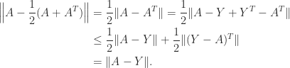


 are the symmetric part and the skew-symmetric part of
  for symmetric
  and skew-symmetric
  . For the
 , and
, and  for any
  such that
  .
. is the nearest Hermitian matrix to
  is the nearest skew-Hermitian matrix to
  -vector
  and returns the vector
  with elements given by
 and
and  , the softmax function is often used to convert a vector
 is the natural logarithm, that is,
  .
. . Note that they are constant on lines
  , as shown by the contours.
 by rewriting it as the exponential of
  and moving it into the numerator, is
 is not recommended, because of the possibility of overflow. Overflow can be avoided in
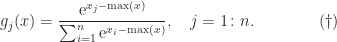
 . It can be shown that computing softmax via this formula is numerically reliable. The shifted version of
  ) is preferred.
 function,
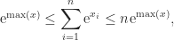

 for
for 
![x = [0~t]^T](https://s0.wp.com/latex.php?latex=x+%3D+%5B0%7Et%5D%5ET&bg=ffffff&fg=222222&s=0&c=20201002) , we obtain the function
, we obtain the function 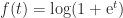 , which is known as the softplus function in machine learning. The softplus function approximates the ReLU (rectified linear unit) activation function
  and satisfies, by
 , in general, we do (trivially) have
  , and more generally
  .
. .
. overflows for
  ,
,  , and
, and  in IEEE half, single, and double precision arithmetic, respectively. Overflow can be avoided by writing
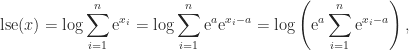
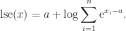
 , so that all exponentiations are of nonpositive numbers and therefore overflow is avoided. Any underflows are harmless. A refinement is to write
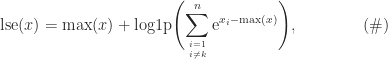
 (if there is more than one such
  , we can take any of them). Here,
  is a function provided in MATLAB and various other languages that accurately evaluates
  even when
  would suffer a loss of precision if it was explicitly computed.
 the shifted formula