What Is the Hilbert Matrix?

The Hilbert matrix $H_n = (h_{ij})$ is the $n\times n$ matrix with $h_{ij} = 1/(i+j-1)$ . For example,

$H_4 = \left[\begin{array}{@{\mskip 5mu}c*{3}{@{\mskip 15mu} c}@{\mskip 5mu}} 1 & \frac{1}{2} & \frac{1}{3} & \frac{1}{4} \\[6pt] \frac{1}{2} & \frac{1}{3} & \frac{1}{4} & \frac{1}{5}\\[6pt] \frac{1}{3} & \frac{1}{4} & \frac{1}{5} & \frac{1}{6}\\[6pt] \frac{1}{4} & \frac{1}{5} & \frac{1}{6} & \frac{1}{7}\\[6pt] \end{array}\right].$

It is probably the most famous test matrix and its conditioning and other properties were extensively studied in the early days of digital computing, especially by John Todd.

The Hilbert matrix is symmetric and it is a Hankel matrix (constant along the anti-diagonals). Less obviously, it is symmetric positive definite (all its eigenvalues are positive) and totally positive (every submatrix has positive determinant). Its condition number grows rapidly with $n$ ; indeed for the 2-norm the asymptotic growth rate is $\kappa_2(H_n) \sim \mathrm{e}^{3.5n}$ . An underlying reason for the ill conditioning is that the Hilbert matrix is obtained when least squares polynomial approximation is done using the monomial basis, and this is known to be an ill-conditioned polynomial basis.

The inverse of $H_n$ has integer entries, with $(i,j)$ entry

$(-1)^{i+j} (i+j-1) \displaystyle{ n+i-1 \choose n-j } { n+j-1 \choose n-i } { i+j-2 \choose i-1 }^2.$

For example,

$H_4^{-1} = \left[\begin{array}{rrrr} 16 & -120 & 240 & -140 \\ -120 & 1200 & -2700 & 1680 \\ 240 & -2700 & 6480 & -4200 \\ -140 & 1680 & -4200 & 2800 \\ \end{array}\right].$

The alternating sign pattern is a consequence of total positivity.

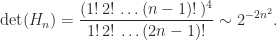
The determinant is also known explicitly:

$\det(H_n) = \displaystyle\frac{ (1!\, 2!\, \dots (n-1)!\, )^4 }{ 1!\, 2!\, \dots (2n-1)! } \sim 2^{-2n^2}. % \cite{todd54}$

The Hilbert matrix is infinitely divisible, which means that the matrix with $(i,j)$ element $h_{ij}^t$ is positive semidefinite for all nonnegative real numbers $t$ .

Other interesting matrices can be formed from the Hilbert matrix. The Lotkin matrix, A = gallery('lotkin',n) in MATLAB, is the Hilbert matrix with the first row replaced by $1$ s, making it nonsymmetric. Like the Hilbert matrix, it is ill conditioned and has an inverse with integer entries. For the $n\times n$ matrix with $(i,j)$ entry $1/(i+j)$ , which is a submatrix of $H_{n+1}$ , the largest singular value tends to $\pi$ as $n\to\infty$ , with error decaying slowly as $O(1/\log n)$ , as was shown by Taussky.

The Hilbert matrix is not a good test matrix, for several reasons. First, it is too ill conditioned, being numerically singular in IEEE double precision arithmetic for $n = 12$ . Second, it is too special: the definiteness and total positivity, together with the fact that it is a special case of a Cauchy matrix (which has elements $1/(x_i + y_j)$ ), mean that certain quantities associated with it can be calculated more accurately than for a general positive definite matrix. The third reason why the Hilbert matrix is not a good test matrix is that most of its elements cannot be stored exactly in floating-point arithmetic, so the matrix actually stored is a perturbation of $H_n$ —and since $H_n$ is ill conditioned this means (for example) that the inverse of the stored matrix can be very different from the exact inverse. A way around this might be to work the integer matrix $H_n^{-1}$ , but its elements are exactly representable in double precision only for $n\le 12$ .

MATLAB has functions hilb and invhilb for the Hilbert matrix and its inverse. How to efficiently form the Hilbert matrix in MATLAB is an interesting question. The hilb function essentially uses the code

j = 1:n;
H = 1./(j'+j-1)

This code is more concise and efficient than two nested loops would be. The second line may appear to be syntactically incorrect, because j'+j adds a column vector to a row vector. However, the MATLAB implicit expansion feature expands j' into an $n\times n$ matrix in which every column is j', expands j into an $n\times n$ matrix in which every row is j, then adds the two matrices. It is not hard to see that the Hilbert matrix is the result of these two lines of code.

References

This is a minimal set of references, which contain further useful references within.

Rajendra Bhatia, Infinitely divisible matrices, Amer. Math. Monthly 113(3), 221–235, 2006.
Man-Duen Choi, Tricks or treats with the Hilbert matrix, Amer. Math. Monthly 90(5), 301–312, 1983
Nicholas J. Higham, Accuracy and Stability of Numerical Algorithms, second edition, Society for Industrial and Applied Mathematics, Philadelphia, PA, USA, 2002. Section 28.1.
M. Lotkin, A set of test matrices, M.T.A.C. 9(52), 153–161, 1955.

Related Blog Posts

Hilbert Matrices by Cleve Moler (2013)
Hilbert Matrices by Cleve Moler (2017)
Implicit Expansion: A Powerful New Feature of MATLAB R2016b (2016)

This article is part of the “What Is” series, available from https://nhigham.com/category/what-is and in PDF form from the GitHub repository https://github.com/higham/what-is.

3 thoughts on “What Is the Hilbert Matrix?”

“the Hilbert matrix is obtained when least squares polynomial approximation is done using the monomial basis”. Could you please clarify? What least squares approximation yields the Hilbert matrix?

Nick Higham says:

July 1, 2020 at 10:36 am

Further details can be found in many numerical analysis textbooks. Try Googling “hilbert matrix normal equations”.

Reply

Dear Michele,
Professor Higham refers to continuous least squares approximation by polynomials, which is not the same thing as polynomial least squares fitting. The entries of the matrix are (definite) integrals of the monomials, when the integration interval is (0,1).
The paper (from 1894) by David Hilbert

“Ein Beitrag zur Theorie des Legendre’schen Polynoms”, Acta Mathematica, 18: 155–159

https://link.springer.com/article/10.1007/BF02418278

seems to be the origin of the name “Hilbert matrix”.

References

Related Blog Posts

Share this:

Related

3 thoughts on “What Is the Hilbert Matrix?”

Leave a Reply Cancel reply