The matrix sign function is the matrix function corresponding to the scalar function of a complex variable

Note that this function is undefined on the imaginary axis. The matrix sign function can be obtained from the Jordan canonical form definition of a matrix function: if 


since all the derivatives of the sign function are zero. The eigenvalues of 


The matrix sign function was introduced by Roberts in 1971 as a tool for model reduction and for solving Lyapunov and algebraic Riccati equations. The fundamental property that Roberts employed is that 


and, writing ![X = [X_1~X_2]](https://s0.wp.com/latex.php?latex=X+%3D+%5BX_1%7EX_2%5D&bg=ffffff&fg=222222&s=0&c=20201002)


![\notag \begin{aligned} \displaystyle\frac{I+S}{2} &= X \begin{bmatrix} 0 & 0 \\ 0 & I_q \end{bmatrix}X^{-1} = X_2 X^{-1}(p+1\colon n,:),\\[\smallskipamount] \displaystyle\frac{I-S}{2} &= X \begin{bmatrix} I_p & 0 \\ 0 & 0 \end{bmatrix}X^{-1} = X_1 X^{-1}(1\colon p,:). \end{aligned}](https://s0.wp.com/latex.php?latex=%5Cnotag+%5Cbegin%7Baligned%7D+++%5Cdisplaystyle%5Cfrac%7BI%2BS%7D%7B2%7D+%26%3D+X+%5Cbegin%7Bbmatrix%7D+0+%26+0+%5C%5C++++++++++++++++++++++++++++++++++++++++++++++++0+++%26+I_q+++++++++++%5Cend%7Bbmatrix%7DX%5E%7B-1%7D+%3D+X_2+X%5E%7B-1%7D%28p%2B1%5Ccolon+n%2C%3A%29%2C%5C%5C%5B%5Csmallskipamount%5D+++%5Cdisplaystyle%5Cfrac%7BI-S%7D%7B2%7D+%26%3D+X+%5Cbegin%7Bbmatrix%7D+I_p+%26+0+%5C%5C++++++++++++++++++++++++++++++++++++++++++++++++++0+++%26+0+++++++++++%5Cend%7Bbmatrix%7DX%5E%7B-1%7D+%3D+X_1+X%5E%7B-1%7D%281%5Ccolon+p%2C%3A%29.+%5Cend%7Baligned%7D+&bg=ffffff&fg=222222&s=0&c=20201002)
Also worth noting are the integral representation

and the concise formula

Application to Sylvester Equation
To see how the matrix sign function can be used, consider the Sylvester equation

This equation is the 

If 


so the solution 
![\bigl[\begin{smallmatrix}A & -C\\ 0& B \end{smallmatrix}\bigr]](https://s0.wp.com/latex.php?latex=%5Cbigl%5B%5Cbegin%7Bsmallmatrix%7DA+%26+-C%5C%5C+0%26+B+%5Cend%7Bsmallmatrix%7D%5Cbigr%5D&bg=ffffff&fg=222222&s=0&c=20201002)


A generalization of this argument shows that the matrix sign function can be used to solve the algebraic Riccati equation 


Application to the Eigenvalue Problem
It is easy to see that 


More generally, for real 


is the number of eigenvalues lying in the vertical strip 
Computing the Matrix Sign Function
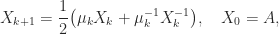
What makes the matrix sign function so interesting and useful is that it can be computed directly without first computing eigenvalues or eigenvectore of

converges quadratically to 
Various other iterations are available for computing

This iteration is quadratically convergent if 
![[1/0]](https://s0.wp.com/latex.php?latex=%5B1%2F0%5D&bg=ffffff&fg=222222&s=0&c=20201002)

where 
![[\ell/m]](https://s0.wp.com/latex.php?latex=%5B%5Cell%2Fm%5D&bg=ffffff&fg=222222&s=0&c=20201002)


Although the rate of convergence of these iterations is at least quadratic, and hence asymptotically fast, it can be slow initially. Indeed for 

with, for example,
This parameter 
As an example, we took A = gallery('lotkin',4), which has eigenvalues 


The Matrix Computation Toolbox contains a MATLAB function signm that computes the matrix sign function. It computes a Schur decomposition then obtains the sign of the triangular Schur factor by a finite recurrence. This function is too expensive for use in applications, but is reliable and is useful for experimentation.
Relation to Matrix Square Root and Polar Decomposition
The matrix sign function is closely connected with the matrix square root and the polar decomposition. This can be seen through the relations
![\notag \mathrm{sign}\left( \begin{bmatrix} 0 & A \\\ I & 0 \end{bmatrix} \right ) = \begin{bmatrix}0 & A^{1/2} \\ A^{-1/2} & 0 \end{bmatrix}, \\[\smallskipamount]](https://s0.wp.com/latex.php?latex=%5Cnotag+++++%5Cmathrm%7Bsign%7D%5Cleft%28+%5Cbegin%7Bbmatrix%7D+0+%26+A+%5C%5C%5C+I+%26+0+%5Cend%7Bbmatrix%7D+%5Cright+%29++++++%3D+%5Cbegin%7Bbmatrix%7D0+%26+A%5E%7B1%2F2%7D+%5C%5C+A%5E%7B-1%2F2%7D+%26+0+%5Cend%7Bbmatrix%7D%2C+%5C%5C%5B%5Csmallskipamount%5D+&bg=ffffff&fg=222222&s=0&c=20201002)
for

for nonsingular 


References
This is a minimal set of references, which contain further useful references within.
- Nicholas J. Higham, Functions of Matrices: Theory and Computation, Society for Industrial and Applied Mathematics, Philadelphia, PA, USA, 2008. (Chapter 5.)
- Charles Kenney and Alan Laub, Rational Iterative Methods for the Matrix Sign Function, SIAM J. Matrix Anal. Appl. 12(2), 273–291, 1991.
- J. D. Roberts, Linear Model Reduction and Solution of the Algebraic Riccati Equation by Use of the Sign Function, Internat. J. Control 32, 677–687, 1980.
Related Blog Posts
- What Is a Matrix Function? (2020)
- What Is a Matrix Square Root? (2020)
- What Is the Polar Decomposition? (2020)
This article is part of the “What Is” series, available from https://nhigham.com/category/what-is and in PDF form from the GitHub repository https://github.com/higham/what-is.
 matrix
  , and it can be written
  . For a rational number
  (where
  and
and  are integers), defining
  is more difficult: is it
  or
or  ? These two possibilities can be different even for
  for an arbitrary real number
  ?
? we define
  , where
  is the principal logarithm: the one taking values in the strip
  . We can generalize this definition to matrices. For a nonsingular matrix
 lie in the strip
 ![\alpha \in [-1,1]](https://s0.wp.com/latex.php?latex=%5Calpha+%5Cin+%5B-1%2C1%5D&bg=ffffff&fg=222222&s=0&c=20201002) , the eigenvalues of
, the eigenvalues of  where
where  is an eigenvalue of
  of the complex plane.
 for a positive integer

 is called the principal
 can be a different matrix. In general, it is not true that
  for real
  , although for symmetric positive definite matrices this identity does hold because the eigenvalues are real and positive.
 is
is
 with
with  is given by the binomial expansion
 real matrices of the form
 there is an explicit formula for
  , where
  . Let
. Let  and
and  . It can be shown that
 can be used computationally, but it is somewhat indirect in that one must approximate both the exponential and the logarithm. A more direct algorithm based on the Schur decomposition and Padé approximation of the power function is developed by Higham and Lin (2013). MATLAB code is available from
  for some nonsingular
  , then
  . This formula is safe to use computationally only if
  then
then  , by the definition of square root. If
  does it follow that
  ? Clearly, the answer is “no” in general because, for example,
  does not imply
  .
. for
for  is the inverse function of
  for
for ![\alpha\in[-1,1]](https://s0.wp.com/latex.php?latex=%5Calpha%5Cin%5B-1%2C1%5D&bg=ffffff&fg=222222&s=0&c=20201002) .
. ? For
? For  , but for real
  such that
 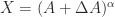 . Assume that
  . Hence the normwise relative backward error is
![\notag \eta(X) = \displaystyle\frac{ \|X^{1/\alpha} - A \|}{\|A\|}, \quad \alpha\in[-1,1].](https://s0.wp.com/latex.php?latex=%5Cnotag++++++%5Ceta%28X%29+%3D+%5Cdisplaystyle%5Cfrac%7B+%5C%7CX%5E%7B1%2F%5Calpha%7D+-+A+%5C%7C%7D%7B%5C%7CA%5C%7C%7D%2C+%5Cquad+%5Calpha%5Cin%5B-1%2C1%5D.+&bg=ffffff&fg=222222&s=0&c=20201002)
 element is the probability of moving from state
  to state
  (years to months) and
  (weeks to days) are among the values of interest. Unfortunately,
 ![\notag A = \left[\begin{array}{ccc} 0 & 1 & 0\\ 0 & 0 & 1\\ 1 & 0 & 0\\ \end{array} \right]](https://s0.wp.com/latex.php?latex=%5Cnotag++++A+%3D+%5Cleft%5B%5Cbegin%7Barray%7D%7Bccc%7D++++++++0++%26+1+%26+0%5C%5C++++++++0++%26+0+%26+1%5C%5C++++++++1++%26+0+%26+0%5C%5C++++++++%5Cend%7Barray%7D+%5Cright%5D+&bg=ffffff&fg=222222&s=0&c=20201002)
![\notag A^{1/2} = \frac{1}{3} \left[\begin{array}{rrr} 2 & 2 & -1 \\ -1 & 2 & 2 \\ 2 & -1 & 2 \end{array} \right],](https://s0.wp.com/latex.php?latex=%5Cnotag++++A%5E%7B1%2F2%7D+%3D+%5Cfrac%7B1%7D%7B3%7D+%5Cleft%5B%5Cbegin%7Barray%7D%7Brrr%7D++++++++2++%26+2+%26+-1+%5C%5C++++++++-1+%26+2+%26+2+%5C%5C++++++++2+%26+-1+%26+2++++++++%5Cend%7Barray%7D+%5Cright%5D%2C+&bg=ffffff&fg=222222&s=0&c=20201002)
![\notag Y = \left[\begin{array}{ccc} 0 & 0 & 1\\ 1 & 0 & 0\\ 0 & 1 & 0\\ \end{array} \right]](https://s0.wp.com/latex.php?latex=%5Cnotag+++++++++Y+%3D+%5Cleft%5B%5Cbegin%7Barray%7D%7Bccc%7D++++++++++0++%26+0++%26++1%5C%5C++++++++++1++%26+0++%26++0%5C%5C++++++++++0++%26+1++%26++0%5C%5C++++++++++%5Cend%7Barray%7D+%5Cright%5D+&bg=ffffff&fg=222222&s=0&c=20201002)
 !)
!)
 , for all
 for some
  with
with  for
for  and
and  ,
,  . Kingman showed in 1962 that this condition holds if and only if for every positive integer
  such that
  .
. , in which case for large problems it is preferable to directly approximate
  or
or  for all
  . Here, the square root is the principal square root (the one lying in the right half-plane) and the logarithm is the principal logarithm (the one with imaginary part in
 ![(-\pi,\pi]](https://s0.wp.com/latex.php?latex=%28-%5Cpi%2C%5Cpi%5D&bg=ffffff&fg=222222&s=0&c=20201002) ).
). by
by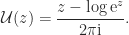
 , in that
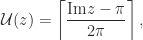
 is the ceiling function, which returns the smallest integer greater than or equal to its argument. It follows that
  if and only if
 ![\mathrm{Im} z \in (-\pi, \pi]](https://s0.wp.com/latex.php?latex=%5Cmathrm%7BIm%7D+z+%5Cin+%28-%5Cpi%2C+%5Cpi%5D&bg=ffffff&fg=222222&s=0&c=20201002) . Hence
. Hence  , replacing
  in
in  ), we have
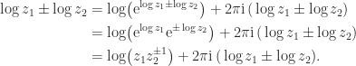

 , in which each occurrence of
  , we have
![\notag f\left( \begin{bmatrix} \lambda_1 & t_{12} \\ 0 & \lambda_2 \end{bmatrix} \right) = \begin{bmatrix} f(\lambda_1) & t_{12} f[\lambda_1,\lambda_2] \\ 0 & f(\lambda_2) \end{bmatrix},](https://s0.wp.com/latex.php?latex=%5Cnotag+++++f%5Cleft%28+%5Cbegin%7Bbmatrix%7D++++++++++++++++++++++%5Clambda_1+%26+t_%7B12%7D++%5C%5C++++++++++++++++++++++++++++0+++%26+%5Clambda_2+++++++++++++%5Cend%7Bbmatrix%7D+%5Cright%29++++++++++%3D+%5Cbegin%7Bbmatrix%7D+++++++++++++++f%28%5Clambda_1%29+%26+t_%7B12%7D+f%5B%5Clambda_1%2C%5Clambda_2%5D+%5C%5C+++++++++++++++++0++++++++++%26+f%28%5Clambda_2%29+++++++++++++%5Cend%7Bbmatrix%7D%2C+&bg=ffffff&fg=222222&s=0&c=20201002)
![\notag f[\lambda_1,\lambda_2] = \begin{cases} \displaystyle\frac{f(\lambda_2)-f(\lambda_1)}{\lambda_2-\lambda_1}, & \lambda_1 \ne \lambda_2, \\ f'(\lambda_1), & \lambda_1 = \lambda_2. \end{cases}](https://s0.wp.com/latex.php?latex=%5Cnotag+++f%5B%5Clambda_1%2C%5Clambda_2%5D++++%3D+%5Cbegin%7Bcases%7D++++++%5Cdisplaystyle%5Cfrac%7Bf%28%5Clambda_2%29-f%28%5Clambda_1%29%7D%7B%5Clambda_2-%5Clambda_1%7D%2C++++++%26+%5Clambda_1+%5Cne+%5Clambda_2%2C+%5C%5C++++++f%27%28%5Clambda_1%29%2C+%26+%5Clambda_1+%3D+%5Clambda_2.+++++%5Cend%7Bcases%7D+&bg=ffffff&fg=222222&s=0&c=20201002)
 this formula suffers from numerical cancellation. For the logarithm, we can rewrite it, using
  , as
, as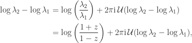
 . Using the hyperbolic arc tangent, defined by
![\notag f[\lambda_1,\lambda_2] = \displaystyle\frac{2\mathrm{atanh}(z) + 2\pi \mathrm{i}\, \mathcal{U}(\log \lambda_2 - \log \lambda_1)}{\lambda_2-\lambda_1}, \quad \lambda_1 \ne \lambda_2.](https://s0.wp.com/latex.php?latex=%5Cnotag+++f%5B%5Clambda_1%2C%5Clambda_2%5D++++%3D+%5Cdisplaystyle%5Cfrac%7B2%5Cmathrm%7Batanh%7D%28z%29+%2B+2%5Cpi+%5Cmathrm%7Bi%7D%5C%2C++++++%5Cmathcal%7BU%7D%28%5Clog+%5Clambda_2+-+%5Clog+%5Clambda_1%29%7D%7B%5Clambda_2-%5Clambda_1%7D%2C++++%5Cquad+%5Clambda_1+%5Cne+%5Clambda_2.+&bg=ffffff&fg=222222&s=0&c=20201002)
 function this formula will provide an accurate value of
 ![f[\lambda_1,\lambda_2]](https://s0.wp.com/latex.php?latex=f%5B%5Clambda_1%2C%5Clambda_2%5D&bg=ffffff&fg=222222&s=0&c=20201002) provided that
provided that  by
by
 if and only if the imaginary parts of all the eigenvalues of
 ![(-\pi, \pi]](https://s0.wp.com/latex.php?latex=%28-%5Cpi%2C+%5Cpi%5D&bg=ffffff&fg=222222&s=0&c=20201002) . Furthermore,
. Furthermore,  is a diagonalizable matrix with integer eigenvalues.
![\notag A = \left[\begin{array}{rrrr} 3 & 1 & -1 & -9\\ -1 & 3 & 9 & -1\\ -1 & -9 & 3 & 1\\ 9 & -1 & -1 & 3 \end{array}\right], \quad \Lambda(A) = \{ 2\pm 8\mathrm{i}, 4 \pm 10\mathrm{i} \}](https://s0.wp.com/latex.php?latex=%5Cnotag+++A+%3D+%5Cleft%5B%5Cbegin%7Barray%7D%7Brrrr%7D++++3+%26+1+%26+-1+%26+-9%5C%5C++++-1+%26+3+%26+9+%26+-1%5C%5C++++-1+%26+-9+%26+3+%26+1%5C%5C++++9+%26+-1+%26+-1+%26+3+%5Cend%7Barray%7D%5Cright%5D%2C++++%5Cquad+%5CLambda%28A%29+%3D+%5C%7B+2%5Cpm+8%5Cmathrm%7Bi%7D%2C+4+%5Cpm+10%5Cmathrm%7Bi%7D+%5C%7D+&bg=ffffff&fg=222222&s=0&c=20201002)
![\notag X = \mathcal{U}(A) = \mathrm{i} \left[\begin{array}{rrrr} 0 & -\frac{1}{2} & 0 & \frac{3}{2}\\ \frac{1}{2} & 0 & -\frac{3}{2} & 0\\ 0 & \frac{3}{2} & 0 & -\frac{1}{2}\\ -\frac{3}{2} & 0 & \frac{1}{2} & 0 \end{array}\right], \quad \Lambda(X) = \{ \pm 1, \pm 2 \}.](https://s0.wp.com/latex.php?latex=%5Cnotag+++X+%3D+%5Cmathcal%7BU%7D%28A%29+%3D+%5Cmathrm%7Bi%7D+%5Cleft%5B%5Cbegin%7Barray%7D%7Brrrr%7D++++0+%26+-%5Cfrac%7B1%7D%7B2%7D+%26+0+%26+%5Cfrac%7B3%7D%7B2%7D%5C%5C++++%5Cfrac%7B1%7D%7B2%7D+%26+0+%26+-%5Cfrac%7B3%7D%7B2%7D+%26+0%5C%5C++++0+%26+%5Cfrac%7B3%7D%7B2%7D+%26+0+%26+-%5Cfrac%7B1%7D%7B2%7D%5C%5C++++-%5Cfrac%7B3%7D%7B2%7D+%26+0+%26+%5Cfrac%7B1%7D%7B2%7D+%26+0+%5Cend%7Barray%7D%5Cright%5D%2C++++%5Cquad+%5CLambda%28X%29+%3D+%5C%7B+%5Cpm+1%2C+%5Cpm+2+%5C%7D.+&bg=ffffff&fg=222222&s=0&c=20201002)
 .
. ,
,

 . If
. If ![\alpha\in(-1,1]](https://s0.wp.com/latex.php?latex=%5Calpha%5Cin%28-1%2C1%5D&bg=ffffff&fg=222222&s=0&c=20201002) and
and  then
then  and so
![\notag (A^\alpha)^{1/\alpha} = A, \quad \alpha \in [-1,1],](https://s0.wp.com/latex.php?latex=%5Cnotag++++++%28A%5E%5Calpha%29%5E%7B1%2F%5Calpha%7D+%3D+A%2C+%5Cquad+%5Calpha+%5Cin+%5B-1%2C1%5D%2C++++&bg=ffffff&fg=222222&s=0&c=20201002)
 , too.
 are nonsingular and
  then
then

![\arg\lambda_i + \arg\mu_i \in(-\pi,\pi]](https://s0.wp.com/latex.php?latex=%5Carg%5Clambda_i+%2B+%5Carg%5Cmu_i+%5Cin%28-%5Cpi%2C%5Cpi%5D&bg=ffffff&fg=222222&s=0&c=20201002) for every eigenvalue
for every eigenvalue  of
of  of
of  .
. ,
,

![(-\pi/2,\pi/2]](https://s0.wp.com/latex.php?latex=%28-%5Cpi%2F2%2C%5Cpi%2F2%5D&bg=ffffff&fg=222222&s=0&c=20201002) then
then  .
.
 , and this equation also holds for
![\mathrm{Im} \lambda \in(-\pi,\pi]](https://s0.wp.com/latex.php?latex=%5Cmathrm%7BIm%7D+%5Clambda+%5Cin%28-%5Cpi%2C%5Cpi%5D&bg=ffffff&fg=222222&s=0&c=20201002) . Using
. Using  in place of
  and
and  . See Aprahamian and Higham (2014) for details.
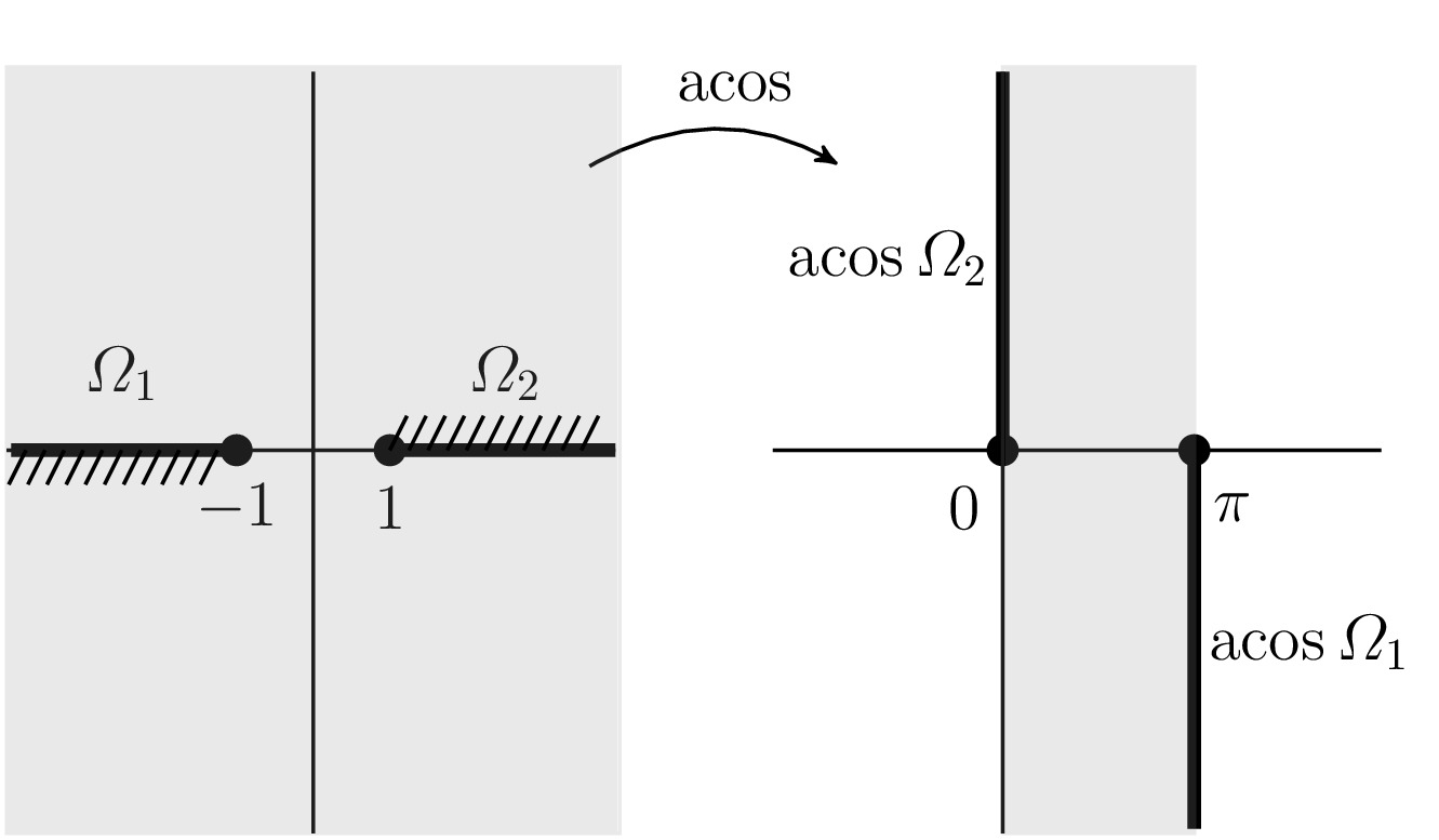
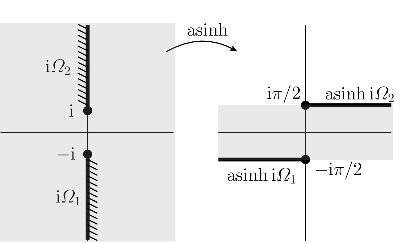
 ? In principle yes, but if the inverse is multivalued the answer is not immediate. The matrix unwinding function is useful for analyzing such round trip relations. As an example, if
  for an integer
 is the principal arc cosine defined in Aprahamian and Higham (2016), where this result and analogous results for the arc sine, arc hyperbolic cosine, and arc hyperbolic sine are derived; and
  is the matrix sign function.
 , where
  is the matrix exponential. Just as in the scalar case, the matrix logarithm is not unique, since if
  for any integer
 identity matrix
  for any
  , whereas the obvious logarithms are the diagonal matrices
  , for integers
  ,
,  , and
, and  . Notice that the repeated eigenvalue
  ,
,  , and
, and  in
in  . This is characteristic of nonprimary logarithms, and in some applications such strange logarithms may be required—an example is the embeddability problem for Markov chains.
 but not for odd
  ,
,![\notag X = \pi\left[\begin{array}{@{}rr@{}} 0 & 1\\ -1 & 0 \end{array}\right]](https://s0.wp.com/latex.php?latex=%5Cnotag++++X+%3D++%5Cpi%5Cleft%5B%5Cbegin%7Barray%7D%7B%40%7B%7Drr%40%7B%7D%7D++++++++++++++0+%26+1%5C%5C++++++++++++++-1+%26+0+++++++++++++%5Cend%7Barray%7D%5Cright%5D+&bg=ffffff&fg=222222&s=0&c=20201002)
 , as does
  for any nonsingular
  , since
  .
. . From this point on we assume that
 ![\notag \begin{aligned} \log A &= \int_0^1 (A-I)\bigl[ t(A-I) + I \bigr]^{-1} \,\mathrm{d}t, \\ \log(I+X) &= X - \frac{X^2}{2} + \frac{X^3}{3} - \frac{X^4}{4} + \cdots, \quad \rho(X)<1, \end{aligned}](https://s0.wp.com/latex.php?latex=%5Cnotag+%5Cbegin%7Baligned%7D+++++++%5Clog+A++%26%3D+%5Cint_0%5E1+%28A-I%29%5Cbigl%5B+t%28A-I%29+%2B+I+%5Cbigr%5D%5E%7B-1%7D+%5C%2C%5Cmathrm%7Bd%7Dt%2C+%5C%5C+++++%5Clog%28I%2BX%29+%26%3D+X+-+%5Cfrac%7BX%5E2%7D%7B2%7D+%2B+%5Cfrac%7BX%5E3%7D%7B3%7D++++++++++++++++++++-+%5Cfrac%7BX%5E4%7D%7B4%7D+%2B+%5Ccdots%2C+%5Cquad+%5Crho%28X%29%3C1%2C+%5Cend%7Baligned%7D+&bg=ffffff&fg=222222&s=0&c=20201002)
 . A useful relation is
  for
for  and
and  (where the square root is the principal square root). Recurring the latter expression gives, for any positive integer
 is small enough that
  can be efficiently approximated by Padé approximation. The MATLAB function
  . Any square root
 , so
, so  is a square root of
  (here, the superscript
  denotes the conjugate transpose).
 then we have
  , so that
  is a square root of
  .
. of a square matrix
  ,
, , where
  .
. satisfies all three conditions.)
 denotes the spectral radius. This definition is natural for functions that have a power series expansion, but it is rather limited in its applicability.
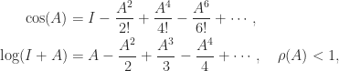

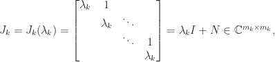


 has the derivatives of
  , where
  is zero apart from a superdiagonal of 1s. The formula for
 : as
: as  we need the existence of the derivatives at
  with
with  .
. that encloses the spectrum of


 .
. and
and  . It is easy to show that
  if
if  for general
 ![[A,B] = AB - BA](https://s0.wp.com/latex.php?latex=%5BA%2CB%5D+%3D+AB+-+BA&bg=ffffff&fg=222222&s=0&c=20201002) . For Hermitian
. For Hermitian  was proved independently by Golden and Thompson in 1965.
 , which is used in the scaling and squaring method for computing the matrix exponential.
 then
then

 , while the solution of the ODE in
  matrices
 .
. ), and they are real if and only if
  , depending on the matrix there can be no square roots, finitely many, or infinitely many. The matrix
 . The identity matrix
 , the lower triangular matrix
![\begin{bmatrix} \cos \theta & \sin \theta \\ \sin \theta & -\cos \theta \end{bmatrix}, \quad \theta \in[0,2\pi]](https://s0.wp.com/latex.php?latex=%5Cbegin%7Bbmatrix%7D++++++%5Ccos+%5Ctheta++%26++%5Csin+%5Ctheta+%5C%5C++++++%5Csin+%5Ctheta++%26+-%5Ccos+%5Ctheta++++++%5Cend%7Bbmatrix%7D%2C+%5Cquad+%5Ctheta+%5Cin%5B0%2C2%5Cpi%5D+&bg=ffffff&fg=222222&s=0&c=20201002)
 above,
  .
. , where
  is also symmetric positive definite.
 square roots, where
  is called a square root, but this is not the standard meaning.
 -matrices,
![G(\theta) = \begin{bmatrix} \cos \theta & \sin \theta \\ -\sin \theta & \cos \theta \end{bmatrix}, \quad \theta \in[0,2\pi],](https://s0.wp.com/latex.php?latex=G%28%5Ctheta%29+%3D+%5Cbegin%7Bbmatrix%7D++++++%5Ccos+%5Ctheta++%26++%5Csin+%5Ctheta+%5C%5C++++++-%5Csin+%5Ctheta++%26+%5Ccos+%5Ctheta++++++%5Cend%7Bbmatrix%7D%2C+%5Cquad+%5Ctheta+%5Cin%5B0%2C2%5Cpi%5D%2C+&bg=ffffff&fg=222222&s=0&c=20201002)
 radians clockwise. The natural square root of
  is
is  . For
. For  , this gives the square root

 , and possibly infinitely many. These two extremes occur when
  , the cost of the recurrence for computing
  is the same as the cost of computing
  , namely
  flops. But while the inverse of a triangular matrix is a level 3 BLAS operation, and so has been very efficiently implemented in libraries, the square root computation is not in the level 3 BLAS standard. As a result, my sqrtm implemented the Björck–Hammarling recurrence in M-code as a triply nested loop and was rather slow.
  , the new code is slower. But for
  we already have a factor 8 speedup, rising to a factor 69 for
  . The slowdown for
 . In this way the task of computing the square root of
  and
and  and then solving the Sylvester equation for
  . The Sylvester equation is solved using an LAPACK routine, for efficiency. If you’d like to take a look at the code, type
 , instead of bounding the
  by
by  , a potentially smaller bound is used.
  and are not willing to compute
  but are willing to compute lower powers of
  , so
, so  ,
,  ,
,  , and
, and  . But it is easy to see that
  and
and  , so we can discard two of the bounds, ending up with
 for values of
 , but
, but 
 , which is a significant improvement.
 the middle term converges to the lower bound, which can be arbitrarily smaller than the upper bound.
 lies in the interval
  is not equivalent to
  for complex
  equal to