Gershgorin Graphics

It’s not so often in numerical linear algebra that the plots we produce are visually attractive. This plot came up in some MATLAB experiments. Can you guess what it is?

I plotted the Gershgorin discs of a stochastic matrix: a matrix with nonnegative elements and row sums all equal to $1$ . The Gershgorin discs for an $n\times n$ matrix $A$ are the $n$ discs in the complex plane defined by

$\notag \Big\{ z\in\mathbb{C}: |z-a_{ii}| \le \displaystyle\sum_{j\ne i} |a_{ij}|\Big\}, \quad i=1\colon n.$

Gershgorin’s theorem says that the eigenvalues of $A$ lie in the union of the discs.

Why do the discs form this interesting pattern? For a stochastic matrix the $i$ th Gershgorin disc is

$\notag \Big\{ z\in\mathbb{C}: |z - a_{ii}| \le \displaystyle\sum_{j\ne i} a_{ij} = 1 - a_{ii} \Big\}.$

This disc goes through $1$ and the closer $a_{ii}$ is to $1$ the smaller the radius of the disc, so the discs are nested, with the disc corresponding to $\min_i a_{ii}$ containing all the others.

The matrix used for the plot is A = anymatrix('core/symmstoch',64) from the Anymatrix collection. It has diagonal elements approximately uniformly distributed on $[0,1]$ , so the centers of the discs are roughly equally spaced and shrink as the centers move to the right.

The image above is for the matrix of dimension $n = 64$ . The black dots are the eigenvalues. Here is the plot for $n = 24$ . The function used to produce these plots is gersh from the Matrix Computation Toolbox.

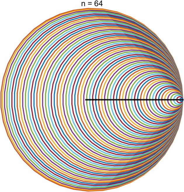
Here are two other matrices whose Gershgorin discs make a graphically interesting plot.

If you know of any other interesting examples please put them in the comments below.

The Big Six Matrix Factorizations

Six matrix factorizations dominate in numerical linear algebra and matrix analysis: for most purposes one of them is sufficient for the task at hand. We summarize them here.

For each factorization we give the cost in flops for the standard method of computation, stating only the highest order terms. We also state the main uses of each factorization.

For full generality we state factorizations for complex matrices. Everything translates to the real case with “Hermitian” and “unitary” replaced by “symmetric” and “orthogonal”, respectively.

The terms “factorization” and “decomposition” are synonymous and it is a matter of convention which is used. Our list comprises three factorization and three decompositions.

Recall that an upper triangular matrix is a matrix of the form

$\notag R = \begin{bmatrix} r_{11} & r_{12} & \dots & r_{1n}\\ & r_{22} & \dots & r_{2n}\\ & & \ddots& \vdots\\ & & & r_{nn} \end{bmatrix},$

and a lower triangular matrix is the transpose of an upper triangular one.

Cholesky Factorization

Every Hermitian positive definite matrix $A\in\mathbb{C}^{n\times n}$ has a unique Cholesky factorization $A = R^*R$ , where $R\in\mathbb{C}^{n\times n}$ is upper triangular with positive diagonal elements.

Cost: $n^3/3$ flops.

Use: solving positive definite linear systems.

LU Factorization

Any matrix $A\in\mathbb{C}^{n\times n}$ has an LU factorization $PA = LU$ , where $P$ is a permutation matrix, $L$ is unit lower triangular (lower triangular with 1s on the diagonal), and $U$ is upper triangular. We can take $P = I$ if the leading principal submatrices $A(1\colon k, 1\colon k)$ , $k = 1\colon n-1$ , of $A$ are nonsingular, but to guarantee that the factorization is numerically stable we need $A$ to have particular properties, such as diagonal dominance. In practical computation we normally choose $P$ using the partial pivoting strategy, which almost always ensures numerically stable.

Cost: $2n^3/3$ flops.

Use: solving general linear systems.

QR Factorization

Any matrix $A\in\mathbb{C}^{m\times n}$ with $m\ge n$ has a QR factorization $A = QR$ , where $Q\in \mathbb{C}^{m\times m}$ is unitary and $R$ is upper trapezoidal, that is, $R = \left[\begin{smallmatrix} R_1 \\ 0\end{smallmatrix}\right]$ , where $R_1\in\mathbb{C}^{n\times n}$ is upper triangular.

Partitioning $Q = [Q_1~Q_2]$ , where $Q_1\in\mathbb{C}^{m\times n}$ has orthonormal columns, gives $A = Q_1R_1$ , which is the reduced, economy size, or thin QR factorization.

Cost: $2(n^2m-n^3/3)$ flops for Householder QR factorization. The explicit formation of $Q$ (which is not usually necessary) requires a further $4(m^2n-mn^2+n^3/3)$ flops.

Use: solving least squares problems, computing an orthonormal basis for the range space of $A$ , orthogonalization.

Schur Decomposition

Any matrix $A\in\mathbb{C}^{n\times n}$ has a Schur decomposition $A = QTQ^*$ , where $Q$ is unitary and $T$ is upper triangular. The eigenvalues of $A$ appear on the diagonal of $T$ . For each $k$ , the leading $k$ columns of $Q$ span an invariant subspace of $A$ .

For real matrices, a special form of this decomposition exists in which all the factors are real. An upper quasi-triangular matrix $R$ is a block upper triangular with whose diagonal blocks $R_{ii}$ are either $1\times1$ or $2\times2$ . Any $A\in\mathbb{R}^{n\times n}$ has a real Schur decomposition $A = Q R Q^T$ , where $Q$ is real orthogonal and $R$ is real upper quasi-triangular with any $2\times2$ diagonal blocks having complex conjugate eigenvalues.

Cost: $25n^3$ flops for $Q$ and $T$ (or $R$ ) by the QR algorithm; $10n^3$ flops for $T$ (or $R$ ) only.

Use: computing eigenvalues and eigenvectors, computing invariant subspaces, evaluating matrix functions.

Spectral Decomposition

Every Hermitian matrix $A\in\mathbb{C}^{n\times n}$ has a spectral decomposition $A = Q\Lambda Q^*$ , where $Q$ is unitary and $\Lambda = \mathrm{diag}(\lambda_i)$ . The $\lambda_i$ are the eigenvalues of $A$ , and they are real. The spectral decomposition is a special case of the Schur decomposition but is of interest in its own right.

Cost: $9n^3$ for $Q$ and $D$ by the QR algorithm, or $4n^3\!/3$ flops for $D$ only.

Use: any problem involving eigenvalues of Hermitian matrices.

Singular Value Decomposition

Any matrix $A\in\mathbb{C}^{m\times n}$ has a singular value decomposition (SVD)

$\notag A = U\Sigma V^*, \quad \Sigma = \mathrm{diag}(\sigma_1,\sigma_2,\dots,\sigma_p) \in \mathbb{R}^{m\times n}, \quad p = \min(m,n),$

where $U\in\mathbb{C}^{m\times m}$ and $V\in\mathbb{C}^{n\times n}$ are unitary and $\sigma_1\ge\sigma_2\ge\cdots\ge\sigma_p\ge0$ . The $\sigma_i$ are the singular values of $A$ , and they are the nonnegative square roots of the $p$ largest eigenvalues of $A^*A$ . The columns of $U$ and $V$ are the left and right singular vectors of $A$ , respectively. The rank of $A$ is equal to the number of nonzero singular values. If $A$ is real, $U$ and $V$ can be taken to be real. The essential SVD information is contained in the compact or economy size SVD $A = U\Sigma V^*$ , where $U\in\mathbb{C}^{m\times r}$ , $\Sigma = \mathrm{diag}(\sigma_1,\dots,\sigma_r)$ , $V\in\mathbb{C}^{n\times r}$ , and $r = \mathrm{rank}(A)$ .

Cost: $14mn^2+8n^3$ for $P(:,1\colon n)$ , $\Sigma$ , and $Q$ by the Golub–Reinsch algorithm, or $6mn^2+20n^3$ with a preliminary QR factorization.

Use: determining matrix rank, solving rank-deficient least squares problems, computing all kinds of subspace information.

Discussion

Pivoting can be incorporated into both Cholesky factorization and QR factorization, giving $\Pi^T A \Pi = R^*R$ (complete pivoting) and $A\Pi = QR$ (column pivoting), respectively, where $\Pi$ is a permutation matrix. These pivoting strategies are useful for problems that are (nearly) rank deficient as they force $R$ to have a zero (or small) $(2,2)$ block.

The big six factorizations can all be computed by numerically stable algorithms. Another important factorization is that provided by the Jordan canonical form, but while it is a useful theoretical tool it cannot in general be computed in a numerically stable way.

For further details of these factorizations see the articles below.

These factorizations are precisely those discussed by Stewart (2000) in his article The Decompositional Approach to Matrix Computation, which explains the benefits of matrix factorizations in numerical linear algebra.

Who Invented the Matrix Condition Number?

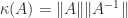
The condition number of a matrix is a well known measure of ill conditioning that has been in use for many years. For an $n\times n$ matrix $A$ it is $\kappa(A) = \|A\| \|A^{-1}\|$ , where $\|\cdot\|$ is any matrix norm. If $A$ is singular we usually regard the condition number as infinite.

The first occurrences of the term “condition number” and of the formula $\kappa(A) = \|A\| \|A^{-1}\|$ that I am aware of are in Turing’s 1948 paper Rounding-Off Errors in Matrix Processes. He defines the $M$ -condition number $n\|A\|_M \|A^{-1}\|_M$ and the $N$ -condition number $n^{-1}\|A\|_F \|A^{-1}\|_F$ , where $\|A\|_M = \max_{i,j}|a_{ij}|$ and $\|A\|_N = (\sum_{i,j}|a_{ij}|^2)^{1/2}$ , the latter N-norm being what we now call the Frobenius norm. He suggests using these condition numbers to measure the ill conditioning of a matrix with respect to linear systems, using a statistical argument to make the connection. He also notes that “the best conditioned matrices are the orthogonal ones”.

In his 1963 book Rounding Errors in Algebraic Processes, Wilkinson credits the first use of “condition number” to Turing and notes that “the term `ill-condition’ had been in common use among numerical analysts for some considerable time before this”. An early mention of linear equations being ill conditioned is in the 1933 paper An Electrical Calculating Machine by Mallock. According to Croarken, Mallock’s machine “could not adequately deal with ill conditioned equations, letting out a very sharp whistle when equilibrium could not be reached”.

As noted by Todd (The Condition of a Certain Matrix, 1950), von Neumann and Goldstine (in their monumental 1947 paper Numerical Inverting of Matrices of High Order) and Wittmeyer (1936) used the ratio of largest to smallest eigenvalue of a positive definite matrix in their analyses, which amounts to the 2-norm condition number $\kappa_2(A) = \|A\|_2 \|A^{-1}\|_2$ , though this formula is not used by these authors. Todd called this the $P$ condition number. None of the $M$ , $N$ or $P$ names have stuck.

Nowadays we know that $\kappa(A)$ can be thought of both as a measure of the sensitivity of the solution of a linear system to perturbations in the data and as a measure of the sensitivity of the matrix inverse to perturbations in the matrix (see, for example, Condition Numbers and Their Condition Numbers by D. J. Higham). How to formulate the definition of condition number for a wide class of problems was worked out by John Rice in his 1966 paper A Theory of Condition.

Empty Matrices in MATLAB

What matrix has zero norm, unit determinant, and is its own inverse? The conventional answer would be that there is no such matrix. But the empty matrix [ ] in MATLAB satisfies these conditions:

>> A = []; norm(A), det(A), inv(A)
ans =
     0
ans =
     1
ans =
     []

While many MATLAB users will be familiar with the use of [ ] as a way of removing a row or column of a matrix (e.g., A(:,1) = []), or omitting an argument in a function call (e.g., max(A,[],2)), fewer will be aware that [ ] is just one in a whole family of empty matrices. Indeed [ ] is the 0-by-0 empty matrix

>> size([])
ans =
     0     0

Empty matrices can have dimension n-by-0 or 0-by-n for any nonnegative integer n. One way to construct them is with double.empty (or the empty method of any other MATLAB class):

>> double.empty
ans =
     []
>> double.empty(4,0)
ans =
   Empty matrix: 4-by-0

What makes empty matrices particularly useful is that they satisfy natural generalizations of the rules of matrix algebra. In particular, matrix multiplicaton is defined whenever the inner dimensions match up.

>> A = double.empty(0,5)*double.empty(5,0)
A =
     []
>> A = double.empty(2,0)*double.empty(0,4)
A =
     0     0     0     0
     0     0     0     0

As the second example shows, the product of empty matrices with positive outer dimensions has zero entries. This ensures that expressions like the following work as we would hope:

>> p = 0; A = ones(3,2); B = ones(3,p); C = ones(2,3); D = ones(p,3);
>> [A B]*[C; D]
ans =
     2     2     2
     2     2     2
     2     2     2

In examples such as this empty matrices are very convenient, as they avoid us having to program around edge cases.

Empty matrices have been in MATLAB since 1986, their inclusion having been suggested by Rod Smart and Rob Schreiber $\lbrack 1 \rbrack$ . A 1989 MATLAB manual says

We’re not sure we’ve done it correctly, or even consistently, but we have found the idea useful.

In those days there was only one empty matrix, the 0-by-0 matrix, and this led Nett and Haddad (1993) to describe the MATLAB implementation of the empty matrix concept as “neither correct, consistent, or useful, at least not for system-theoretic applications”. Nowadays MATLAB gets it right and indeed it adheres to the rules suggested by those authors and by de Boor (1990). If you are wondering how the values for norm([]), det([]) and inv([]) given above are obtained, see de Boor’s article for an explanation in terms of linear algebra transformations.

The concept of empty matrices dates back to before MATLAB. The earliest reference I am aware of is a 1970 book by Stoer and Witzgall. As the extract below shows, these authors recognized the need to support empty matrices of varying dimension and they understood how multiplication of empty matrices should work.

Reference

John N. Little, The MathWorks Newsletter, 1 (1), March 1986.

Faster SVD via Polar Decomposition

The car number plate of Gene Golub, who did so much to promote the SVD. Photo credit: P. M. Kroonenberg.

The singular value decomposition (SVD) is one of the most important tools in matrix theory and matrix computations. It is described in many textbooks and is provided in all the standard numerical computing packages. I wrote a two-page article about the SVD for The Princeton Companion to Applied Mathematics, which can be downloaded in pre-publication form as an EPrint.

The polar decomposition is a close cousin of the SVD. While it is probably less well known it also deserves recognition as a fundamental theoretical and computational tool. The polar decomposition is the natural generalization to matrices of the polar form $z = r \mathrm{e}^{\mathrm{i}\theta}$ for complex numbers, where $r\ge0$ , $\mathrm{i}$ is the imaginary unit, and $\theta\in(-\pi,\pi]$ . The generalization to an $m\times n$ matrix is $A = UH$ , where $U$ is $m\times n$ with orthonormal columns and $H$ is $n\times n$ and Hermitian positive semidefinite. Here, $U$ plays the role of $\mathrm{e}^{\mathrm{i}\theta}$ in the scalar case and $H$ the role of $r$ .

It is easy to prove existence and uniqueness of the polar decomposition when $A$ has full rank. Since $A = UH$ implies $A^*A = HU^*UH = H^2$ , we see that $H$ must be the Hermitian positive definite square root of the Hermitian positive definite matrix $A^*A$ . Therefore we set $H = (A^*A)^{1/2}$ , after which $U = AH^{-1}$ is forced. It just remains to check that this $U$ has orthonormal columns: $U^*U = H^{-1}A^*AH^{-1} = H^{-1}H^2H^{-1} = I$ .

Many applications of the polar decomposition stem from a best approximation property: for any $m\times n$ matrix $A$ the nearest matrix with orthonormal columns is the polar factor $U$ , for distance measured in the 2-norm, the Frobenius norm, or indeed any unitarily invariant norm. This result is useful in applications where a matrix that should be unitary turns out not to be so because of errors of various kinds: one simply replaces the matrix by its unitary polar factor.

However, a more trivial property of the polar decomposition is also proving to be important. Suppose we are given $A = UH$ and we compute the eigenvalue decomposition $H = QDQ^*$ , where $D$ is diagonal with the eigenvalues of $H$ on its diagonal and $Q$ is a unitary matrix of eigenvectors. Then $A = UH = UQDQ^* = (UQ)DQ^* \equiv P\Sigma Q^*$ is an SVD! My PhD student Pythagoras Papadimitriou and I proposed using this relation to compute the SVD in 1994, and obtained speedups by a factor six over the LAPACK SVD code on the Kendall Square KSR1, a shared memory parallel machine of the time.

Yuji Nakatsukasa and I recently revisited this idea. In a 2013 paper in the SIAM Journal of Scientific Computing we showed that on modern architectures it is possible to compute the SVD via the polar decomposition in a way that is both numerically stable and potentially much faster than the standard Golub–Reinsch SVD algorithm. Our algorithm has two main steps.

Compute the polar decomposition by an accelerated Halley algorithm called QDWH devised by Nakatsukasa, Bai, and Gygi (2010), for which the main computational kernel is QR factorization.
Compute the eigendecomposition of the Hermitian polar factor by a spectral divide and conquer algorithm. This algorithm repeatedly applies QDWH to the current block to compute an invariant subspace corresponding to the positive or negative eigenvalues and thereby divides the problem into two smaller pieces.

The polar decomposition is fundamental to both steps of the algorithm. While the total number of flops required is greater than for the standard SVD algorithm, the new algorithm has lower communication costs and so should be faster on parallel computing architectures once communication costs are sufficiently greater than the costs of floating point arithmetic. Sukkari, Ltaief, and Keyes have recently shown that on a multicore architecture enhanced with multiple GPUs the new QDWH-based algorithm is indeed faster than the standard approach. Another interesting feature of the new algorithm is that it has been found experimentally to have better accuracy.

The Halley iteration that underlies the QDWH algorithm for the polar decomposition has cubic convergence. A version of QDWH with order of convergence seventeen, which requires just two iterations to converge to double-precision accuracy, has been developed by Nakatsukasa and Freund (2015), and is aimed particularly at parallel architectures. This is a rare example of an iteration with a very high order of convergence actually being of practical use.

Numerical Linear Algebra and Matrix Analysis

Matrix analysis and numerical linear algebra are two very active, and closely related, areas of research. Matrix analysis can be defined as the theory of matrices with a focus on aspects relevant to other areas of mathematics, while numerical linear algebra (also called matrix computations) is concerned with the construction and analysis of algorithms for solving matrix problems, as well as related topics such as problem sensitivity and rounding error analysis.

My article Numerical Linear Algebra and Matrix Analysis for The Princeton Companion to Applied Mathematics gives a selective overview of these two topics. The table of contents is as follows.

1 Nonsingularity and Conditioning
2 Matrix Factorizations
3 Distance to Singularity and Low-Rank Perturbations
4 Computational Cost
5 Eigenvalue Problems
  5.1 Bounds and Localization
  5.2 Eigenvalue Sensitivity
  5.3 Companion Matrices and the Characteristic Polynomial
  5.4 Eigenvalue Inequalities for Hermitian Matrices
  5.5 Solving the Non-Hermitian Eigenproblem
  5.6 Solving the Hermitian Eigenproblem
  5.7 Computing the SVD
  5.8 Generalized Eigenproblems
6 Sparse Linear Systems
7 Overdetermined and Underdetermined Systems
  7.1 The Linear Least Squares Problem
  7.2 Underdetermined Systems
  7.3 Pseudoinverse
8 Numerical Considerations
9 Iterative Methods
10 Nonnormality and Pseudospectra
11 Structured Matrices
  11.1 Nonnegative Matrices
  11.2 M-Matrices
12 Matrix Inequalities
13 Library Software
14 Outlook

The article can be downloaded in pre-publication form as an EPrint.

1980s Microcomputers and the LINPACK Benchmark

As an undergraduate and postgraduate student in the early 1980s I owned a Commodore Pet microcomputer and then a Commodore 64. Both came with Basic built into ROM. On booting the machines you were presented with a flashing cursor and could type in programs to be executed by the Basic interpreter or load programs from cassette or disk.

I used the machines in my research on matrix computations, writing many programs in Basic and Comal (a more structured, Pascal-like version of Basic, originating in Denmark).

Recently, I was looking for information about the microprocessors used in the early microcomputers. I could not find what I wanted, but remembered that some relevant information is contained in the appendices of a technical report Matrix Computations in Basic on a Microcomputer that I wrote in 1985 (the published version ¹ omits the appendices). Specifically, the appendices contain

specifications of the Commodore 64, the BBC Microcomputer Model B and Model B with Torch Z-80 second processor, and the Amstrad CPC-64,
examples of 6502 assembly language programs for the Commodore 64 and the BBC Model B,
Basic and Comal programs for the above machines.

As these are of some historical interest I have scanned the technical report and made it available as a MIMS EPrint. I still have the original hard copy, which was produced on the Commodore 64 itself using a wordprocessor called Vizawrite 64 and printed on an Epson FX-80 dot matrix printer, taking advantage of the printer’s ability to produce subscripts. These were the days before TeX was widely available, and looking back I am surprised that I was able to produce such a neatly formatted document, with tables and program listings. Just printing it must have taken a few hours. Vizawrite was the last wordprocessor I have used seriously, and adapting Tony Hoare’s quote about Algol I would say that it was “so far ahead of its time that it was not only an improvement on its predecessors but also on nearly all its successors”.

The purpose of the report was to convert the LINPACK Fortran linear equation solvers SGEFA/SGESL to Basic and run them on the four machines mentioned above. I found that the cost of the computations was dominated by subscripting calculations and not the floating point arithmetic. I therefore translated the Basic Linear Algebra Subprograms (BLAS) that are called by the codes into assembly language for the Commodore and BBC machines and obtained significant speedups, due to removal of the subscripting overheads.

Writing in assembly language is very different from writing in a high-level language, because the available operations are so simple: load the contents of a memory location into the accumulator, increment or decrement by one the value stored in a memory location, and so on. Fortunately, when I started this project I already had experience of writing 6502 assembly language as I had used it in my Music Master program for the Commodore 64 published by Supersoft. And I had the excellent Mikro Assembler cartridge for the Commodore 64 that made developing assembly code as easy and enjoyable as it could be.

The LINPACK routines that I translated are the ones originally used for the LINPACK benchmark that has been used since the 1980s to measure the speed of the world’s fastest computers. Based on the timings in my article extrapolated to 100 by 100 matrices, here is a table comparing the speed in megaflops of the Commodore and BBC machines with that of two recent low-end computers:

Machine	Year	Megaflops
Commodore 64 (Basic + machine code)	1985	0.0005
BBC Model B (Basic + machine code)	1985	0.0008
iPad 2 (data from Jack Dongarra)	2011	620
Raspberry Pi	2013	42

Footnotes:

N. J. Higham. Matrix computations in Basic on a microcomputer. IMA Bulletin, 22:13-20, 1986.

The Nearest Correlation Matrix

A correlation matrix is a symmetric matrix with unit diagonal and nonnegative eigenvalues. In 2000 I was approached by a London fund management company who wanted to find the nearest correlation matrix (NCM) in the Frobenius norm to an almost correlation matrix: a symmetric matrix having a significant number of (small) negative eigenvalues. This problem arises when the data from which the correlations are constructed is asynchronous or incomplete, or when models are stress-tested by artificially adjusting individual correlations. Solving the NCM problem (or obtaining a true correlation matrix some other way) is important in order to avoid subsequent calculations breaking down due to negative variances or volatilities, for example.

Algorithms

The convexity properties of the problem mean that there is a unique nearest correlation matrix, which is hence a global minimizer. In the 1990s several algorithms had been proposed for computing it, but none was guaranteed to work. Prompted by the approach from the company, I investigated the problem. I proved some results characterizing the solution and derived an alternating projections algorithm for computing it ¹. The algorithm repeatedly projects onto the set of matrices with unit diagonal and the cone of symmetric positive semidefinite matrices. It is guaranteed to converge to the minimum, but does so at a linear rate. An important feature of the algorithm is that other projections can be added on. Thus, for example, if we want to leave the trailing principal submatrix of order three unchanged, we simply restore it at the end of each iteration ², ³.

The alternating projections algorithm is widely used, but can be slow to converge, especially for large matrices ⁴. In 2006, Qi and Sun ⁵ derived a Newton method for the NCM problem. They work with the dual of the original problem, which is unconstrained. The objective function of the dual is not twice continuously differentiable, but by using the theory of strongly semismooth matrix functions Qi and Sun show that Newton’s method nevertheless has global quadratic convergence.

Ruediger Borsdorf and I, building on work in his M.Sc. thesis ³, built an algorithm that solves the Newton equations using minres with a Jacobi preconditioner (a nontrivial task since the coefficient matrix is not explicitly available), and has some other refinements described in ⁶. This algorithm has been implemented in the NAG Library ⁷.

In subsequent work, Borsdorf, Marcos Raydan and I ⁸ ^,⁹ used the spectral projected gradient method (SPGM) to solve the k-factor NCM, in which the correlation matrix is constrained to have the form of a diagonal matrix plus a rank-k matrix. This problem variant arises in multifactor normal copula models, collateralized debt obligations (CDOs), and multivariate time series. One existing previous algorithm can fail to converge or solve the problem, but the SPGM has guaranteed convergence to a stationary point. This algorithm has also been implemented in the NAG Library.

The NCM problem has proved to be of very wide interest beyond the world of finance, as indicated by the fact that ¹ is now my third best cited paper on the Web of Science. Recent applications in which the problem arises include reconstructing 20th century sea levels, genetic evaluations for thoroughbred horse breeding, modelling public health data sets, modelling storm damage of buildings, and a Kriging model for reservoirs.

Software

I regularly receive emails asking for software implementing algorithms for the NCM problem. I thought it would be useful to summarize what is available. In general, the Newton method is preferred, but the alternating projections method is more flexible as regards incorporating additional constraints.

Original NCM Problem

Alternating Projections Method

MATLAB: Craig Lucas, near_cor.
MATLAB: Erlend Ringstad, validcorr.
MATLAB: Nick Higham, nearcorr (see below).
Python: Mike Croucher, nearest_correlation.
R: Jens Oehlschlaegel and R Matrix package authors, nearPD.
SAS: Rick Wicklin, NearestCorr.

Newton Method

MATLAB: Defeng Sun, various codes.
NAG Library (Fortran/SMP, C, NAG Toolbox for MATLAB, .NET, Java, Excel, R, Python):
- g02aaf (Fortran), g02aac (C), g02aa.m (MATLAB), g02aa (R),
- g02abf (Fortran), g02abc (C), g02abm (MATLAB), g02ab (R): allows for weighted Frobenius norm based on two-sided scaling and lower bounds on the eigenvalues.
- g02ajf (Fortran), g02ajc (C), g02ajf.m (MATLAB): allows for componentwise weighted Frobenius norm and lower bounds on the eigenvalues.

k-Factor NCM Problem

NAG Library (Fortran/SMP, C, NAG Toolbox for MATLAB, .NET, Java, Excel, R, Python):)
- g02aef (Fortran), g02aec (C), g02ae.m (MATLAB), g02ae (R).

A MATLAB Alternating Projections Function

I thought it would be useful to provide my own MATLAB function nearcorr.m implementing the alternating projections algorithm. The listing is below. To see how it compares with the NAG code g02aa.m I ran the test code

%NEARCORR_TEST  Compare g02aa and nearcorr.

rng(10)                                  % Seed random number generators.
n = 100;
A = gallery('randcorr',n);               % Random correlation matrix. 
E  = randn(n)*1e-1;  A = A + (E + E')/2; % Perturb it.
tol = 1e-10;

% A = cor1399; tol = 1e-4;

fprintf('g02aa:\n')
maxits = int64(-1);  % For linear equation solver.
maxit = int64(-1);   % For Newton iteration.
tic
[~,X1,iter1,feval,nrmgrd,ifail] = g02aa(A,'errtol',tol,'maxits',maxits, ...
                                          'maxit',maxit);
toc

fprintf('  Newton steps taken: %d\n', iter1);
fprintf('  Norm of gradient of last Newton step: %6.4f\n', nrmgrd);
if ifail > 0, fprintf('  g02aa failed with ifail = %g\n', ifail), end

fprintf('nearcorr:\n')
tic
[X2,iter2] = nearcorr(A,tol,[],[],[],[],1);
toc
fprintf('  Number of iterations: %d\n', iter2);

fprintf('  Normwise relative difference between computed solutions:')
fprintf('%9.2e\n', norm(X1-X2,1)/norm(X1,1))

Running under Windows 7 on an Ivy Bridge Core i7 processor @4.4Ghz I obtained the following results, where the “real-life” matrix is based on stock data:

Matrix	Code	Time (secs)	Iterations
1. Random (100), tol = 1e-10	g02aa	0.023	4
	nearcorr	0.052	15
2. Random (500), tol = 1e-10	g02aa	0.48	4
	nearcorr	3.01	26
3. Real-life (1399), tol = 1e-4	g02aa	6.8	5
	nearcorr	100.6	68

The results show that while nearcorr can be fast for small dimensions, the number of iterations, and hence its run time, tends to increase with the dimension and it can be many times slower than the Newton method. This is a stark illustration of the difference between quadratic convergence and linear (with problem-dependent constant) convergence. Here is my MATLAB function nearcorr.m.

function [X,iter] = nearcorr(A,tol,flag,maxits,n_pos_eig,w,prnt)
%NEARCORR    Nearest correlation matrix.
%   X = NEARCORR(A,TOL,FLAG,MAXITS,N_POS_EIG,W,PRNT)
%   finds the nearest correlation matrix to the symmetric matrix A.
%   TOL is a convergence tolerance, which defaults to 16*EPS.
%   If using FLAG == 1, TOL must be a 2-vector, with first component
%   the convergence tolerance and second component a tolerance
%   for defining "sufficiently positive" eigenvalues.
%   FLAG = 0: solve using full eigendecomposition (EIG).
%   FLAG = 1: treat as "highly non-positive definite A" and solve
%             using partial eigendecomposition (EIGS).
%   MAXITS is the maximum number of iterations (default 100, but may
%   need to be increased).
%   N_POS_EIG (optional) is the known number of positive eigenvalues of A.
%   W is a vector defining a diagonal weight matrix diag(W).
%   PRNT = 1 for display of intermediate output.

%   By N. J. Higham, 13/6/01, updated 30/1/13, 15/11/14, 07/06/15.
%   Reference:  N. J. Higham, Computing the nearest correlation
%   matrix---A problem from finance. IMA J. Numer. Anal.,
%   22(3):329-343, 2002.

if ~isequal(A,A'), error('A must by symmetric.'), end
if nargin < 2 || isempty(tol), tol = length(A)*eps*[1 1]; end
if nargin < 3 || isempty(flag), flag = 0; end
if nargin < 4 || isempty(maxits), maxits = 100; end
if nargin < 6 || isempty(w), w = ones(length(A),1); end
if nargin < 7, prnt = 1; end

n = length(A);
if flag >= 1
   if nargin < 5 || isempty(n_pos_eig)
      [V,D] = eig(A); d = diag(D);
      n_pos_eig = sum(d >= tol(2)*d(n));
   end
   if prnt, fprintf('n = %g, n_pos_eig = %g\n', n, n_pos_eig), end
end

X = A; Y = A;
iter = 0;
rel_diffX = inf; rel_diffY = inf; rel_diffXY = inf;
dS = zeros(size(A));

w = w(:); Whalf = sqrt(w*w');

while max([rel_diffX rel_diffY rel_diffXY]) > tol(1)

   Xold = X;
   R = Y - dS;
   R_wtd = Whalf.*R;
   if flag == 0
      X = proj_spd(R_wtd);
   elseif flag == 1
      [X,np] = proj_spd_eigs(R_wtd,n_pos_eig,tol(2));
   end
   X = X ./ Whalf;
   dS = X - R;
   Yold = Y;
   Y = proj_unitdiag(X);
   rel_diffX = norm(X-Xold,'fro')/norm(X,'fro');
   rel_diffY = norm(Y-Yold,'fro')/norm(Y,'fro');
   rel_diffXY = norm(Y-X,'fro')/norm(Y,'fro');
   iter = iter + 1;
   if prnt
      fprintf('%2.0f:  %9.2e  %9.2e  %9.2e', ...
               iter, rel_diffX, rel_diffY, rel_diffXY)
      if flag >= 1, fprintf('  np = %g\n',np), else fprintf('\n'), end
   end
   if iter > maxits
       error(['Stopped after ' num2str(maxits) ' its. Try increasing MAXITS.'])
   end

end

%%%%%%%%%%%%%%%%%%%%%%%%
function A = proj_spd(A)
%PROJ_SPD

if ~isequal(A,A'), error('Not symmetric!'), end
[V,D] = eig(A);
A = V*diag(max(diag(D),0))*V';
A = (A+A')/2; % Ensure symmetry.

%%%%%%%%%%%%%%%%%%%%%%%%%%%%%%%%%%%%%%%%%%%%%%%%%%%%%%%%%%%%%
function [A,n_pos_eig_found] = proj_spd_eigs(A,n_pos_eig,tol)
%PROJ_SPD_EIGS

if ~isequal(A,A'), error('Not symmetric!'), end
k = n_pos_eig + 10; % 10 is safety factor.
if k > length(A), k = n_pos_eig; end
opts.disp = 0;
[V,D] = eigs(A,k,'LA',opts); d = diag(D);
j = (d > tol*max(d));
n_pos_eig_found = sum(j);
A = V(:,j)*D(j,j)*V(:,j)';  % Build using only the selected eigenpairs.
A = (A+A')/2; % Ensure symmetry.

%%%%%%%%%%%%%%%%%%%%%%%%%%%%%
function A = proj_unitdiag(A)
%PROJ_SPD

n = length(A);
A(1:n+1:n^2) = 1;

Updates

Links updated August 4, 2014.
nearcorr.m corrected November 15, 2014: iter was incorrectly initialized (thanks to Mike Croucher for pointing this out).
Added link to Mike Croucher’s Python alternating directions code, November 17, 2014.
Corrected an error in the convergence test, June 7, 2015. Effect on performance will be minimal (thanks to Nataša Strabić for pointing this out).

Footnotes:

Nicholas J. Higham, Computing the Nearest Correlation Matrix—A Problem from Finance, IMA J. Numer. Anal. 22, 329–343, 2002.

Craig Lucas, Computing Nearest Covariance and Correlation Matrices, M.Sc. Thesis, University of Manchester, 2001.

Ruediger Borsdorf, A Newton Algorithm for the Nearest Correlation Matrix, M.Sc. Thesis, University of Manchester, 2007.

⁴

Rene Escalante and Marcos Raydan, Alternating Projection Methods, SIAM, 2011.

⁵

Hou-Duo Qi and Defeng Sun, A Quadratically Convergent Newton Method for Computing the Nearest Correlation Matrix, SIAM J. Matrix Anal. Appl. 28, 360-385, 2006

⁶

Ruediger Borsdorf and Nicholas J. Higham, A Preconditioned Newton Algorithm for the Nearest Correlation Matrix, IMA J. Numer. Anal. 30, 94-107, 2010.

⁷

Nearest Correlation Matrix (Mark 22) and Additions to Nearest Correlation Matrix (Mark 23), NAG Ltd.

⁸

Ruediger Borsdorf, Nicholas Higham and Marcos Raydan, Computing a Nearest Correlation Matrix with Factor Structure, SIAM J. Matrix Anal., Appl. 31, 2603-2622, 2010

⁹

Ruediger Borsdorf, Structured Matrix Nearness Problems: Theory and Algorithms, Ph.D. Thesis, University of Manchester, 2012.

Category: matrix computations

Gershgorin Graphics

Related Blog Posts

The Big Six Matrix Factorizations

Cholesky Factorization

LU Factorization

QR Factorization

Schur Decomposition

Spectral Decomposition

Singular Value Decomposition

Discussion

Related Blog Posts

Who Invented the Matrix Condition Number?

Empty Matrices in MATLAB

Reference

Faster SVD via Polar Decomposition

Numerical Linear Algebra and Matrix Analysis

1980s Microcomputers and the LINPACK Benchmark

Footnotes:

The Nearest Correlation Matrix

Algorithms

Software

Original NCM Problem

Alternating Projections Method

Newton Method

k-Factor NCM Problem

A MATLAB Alternating Projections Function

Footnotes:

Related Blog Posts

Share this:

Cholesky Factorization

LU Factorization

QR Factorization

Schur Decomposition

Spectral Decomposition

Singular Value Decomposition

Discussion

Related Blog Posts

Share this:

Share this:

Reference

Share this:

Share this:

Share this:

Footnotes:

Share this:

Algorithms

Software

Original NCM Problem

Alternating Projections Method

Newton Method

k-Factor NCM Problem

A MATLAB Alternating Projections Function

Footnotes:

Share this: