By Len Freeman, Nick Higham and Jim Nagy.

Ian Gladwell passed away on May 23, 2021 at the age of 76. He was born in Bolton, Lancashire in 1944. He did his secondary education at Thornleigh College, Bolton and was an undergraduate at Hertford College, University of Oxford, from where he graduated with a B.A. Hons. in Mathematics in 1966. He did his postgraduate studies at the University of Manchester, gaining an MSc in Numerical Analysis and Computing in 1967 and a PhD in Numerical Analysis in 1970. He was the first PhD student of Christopher T. H. Baker (1939–2017).
Ian was appointed Lecturer in the Department of Mathematics at the University of Manchester in 1969 and progressed to Senior Lecturer in 1980. He was a member of the Numerical Analysis Group (along with Christopher Baker, Len Freeman, George Hall, Will McLewin, Jack Williams (1943–2015), and Joan Walsh (1932–2017)) who, together with colleagues at UMIST, made Manchester a major centre of numerical analysis activity from the 1970s onwards.
Ian’s research focused on ordinary differential equation (ODE) initial value problems and boundary value problems, mathematical software, and parallel computing, and he had a wide knowledge of numerical analysis and scientific computing. He was perhaps best known for his pioneering work on mathematical software for the numerical solution of ODEs, much of which was published in the NAG Library and in the journal ACM Transactions on Mathematical Software. A particular topic of interest for Ian was algorithms and software for the numerical solution of almost block diagonal linear systems, which arise in discretizations of boundary value problems for ODEs and partial differential equations.
More details on Ian’s publications can be found at his MathSciNet author profile (subscription required). It lists 55 publications with 19 co-authors, among which Richard Brankin, Larry Shampine, Ruth Thomas, and Marcin Paprzycki are his most frequent co-authors.
In his time at Manchester he collaborated with a variety of colleagues both inside and outside the department, and he was always ready to offer advice to students and colleagues across the campus on numerical computing (as evidenced by the common sight of people waiting outside his office door to be seen).
Ian was instrumental in setting up the Manchester Numerical Analysis Reports, a long-running technical report series to which he contributed many items.
Ian had a five-month visit to the Department of Computer Science at the University of Toronto in 1975. Links between the Manchester and Toronto departments were strong, and over the years numerical analysts made several visits in both directions.
In the mid 1980s, Ian was one of the first people in the UK to have an email address: igladwel@uk.ac.ucl.cs. His email account was on a computer at University College London (UCL), because UCL hosted a gateway between JANET, the UK computer network, and ARPANET in the USA. Ian kindly allowed Nick Higham and Len Freeman use of the account to communicate with colleagues in the US.
Ian had long-standing collaborations with the Numerical Algorithms Group (NAG) Ltd., Oxford. He contributed many codes and associated documentation to the NAG Library, principally in ordinary differential equations. In a 1979 paper in ACM Trans. Math. Software he wrote
“When the NAG library structure was designed in the late 1960s, it was decided to devote a chapter, named DO2, to the numerical solution of systems of ordinary differential equations and that this chapter would be contributed by members of the Department of Mathematics, University of Manchester, and in particular by J. E. Walsh, G. Hall, and the author.”
Ian was a long-term member of NAG and of the NAG Technical Policy Committee, and during 1986 he held a Royal Society/Science and Engineering Research Council Industrial Fellowship at NAG.
Nick Higham was taught by Ian in an upper level undergraduate course “Numerical Linear Algebra” that Ian was giving for the first time, in 1981. As an MSc student and PhD student he benefited greatly from Ian’s advice about how to think about and do research.
Ian moved to the Department of Mathematics at Southern Methodist University (SMU), Dallas, as a Visiting Associate Professor in 1987, which became a permanent position in 1988. He had collaborated during the 1980s with Larry Shampine, who was working at Sandia National Laboratories until he moved to the SMU Mathematics Department in 1986.
Ian served as chair of the department 1988–1994 and again in 1998. He was also Director of Graduate Studies from 2005–2008. Ian excelled in these roles as mentor, which is recognized by a PhD fellowship in his honor. Jim Nagy was extremely fortunate to have Ian as his first department chair in 1992; Ian mentored him during the challenging tenure-track years, advising on research, teaching and more, including extensive editing of his first successful grant proposals.
Ian wrote the book Solving ODEs with MATLAB (2003) with Larry Shampine and Skip Thompson, which was described as “an excellent treatment of the fundamentals for solving ODEs using MATLAB” in Mathematical Reviews. It is Ian’s most highly cited work, with around 900 citations on Google Scholar at the time of writing.
Ian served as editor for ten journals, including as Associate Editor (2002–2005) and Editor-in-Chief (2005–2008) of ACM Transactions on Mathematical Software, as Associate Editor of the IMA Journal on Numerical Analysis (1988–2007), and as Associate Editor of Scalable Computing: Practice and Experience (2005–2010). A special issue of the latter journal in 2009 was dedicated to him on the occasion of his retirement from SMU
Ian was a long-term member of the Institute of Mathematics and Its Applications, of which he was a Fellow, and the Society for Industrial and Applied Mathematics.
According to the Mathematics Genealogy Project, Ian had 23 PhD students, equally split between Manchester and SMU, with one jointly supervised at the University of Bari.
 matrix
  is defined by
 permutations
  ) of the sequence
  and
and  is the number of inversions in
  , that is, the number of pairs
  with
with  . Each term in the sum is a signed product of
  entries of
  .
.

 , where
  denotes the
  submatrix of
  and column
  for a scalar
  . This formula is called the expansion by minors because
  is a minor of
  is triangular then
  . If
. If  is unitary then
  implies
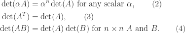
  on using (3) and (4). An
  of
of  . Since the eigenvalues are the roots of the characteristic polynomial
  , this relation follows by setting
  in the expression
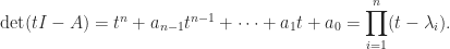
 , the determinant is
 the determinant is tedious to write down. If one must compute
  , the formulas (1) and (5) are too expensive unless
  is an LU factorization, with
  a permutation matrix,
  unit lower triangular, and
  upper triangular, then
  . As this expression indicates, the determinant is prone to overflow and underflow in floating-point arithmetic, so it may be preferable to compute
  .
.
 is the
  element
  ). More generally, Cramer’s rule says that the components of the solution to a linear system
  are given by
  , where
  denotes
  . While mathematically elegant, Cramer’s rule is of no practical use, as it is both expensive and numerically unstable in finite precision arithmetic.
 is Hadamard’s inequality. Note that for such
  ,
,  is real and positive (being the product of the eigenvalues, which are real and positive) and the diagonal elements are also real and positive (since
  ).
).
 or by using a QR factorization of
 ![A = [a_1,a_2,\dots,a_n] \in\mathbb{C}^{n\times n}](https://s0.wp.com/latex.php?latex=A+%3D+%5Ba_1%2Ca_2%2C%5Cdots%2Ca_n%5D+%5Cin%5Cmathbb%7BC%7D%5E%7Bn%5Ctimes+n%7D&bg=ffffff&fg=222222&s=0&c=20201002) ,
,
 and obtain the analogous bound with column norms replaced by row norms.
 can be interpreted as the volume of the parallelepiped
  , whose sides are the columns of
  . It might be tempting to use
  as a measure of how close a nonsingular matrix
  can be given any value by a suitable choice of
  , yet
, yet  is perfectly conditioned:
  , where
  is the condition number.
 and
and  if and only if the columns of
  the Hadamard condition number. In general,
  , but if
  -norm then it can be shown that
  (Higham, 2002, Prob. 14.13). Dixon (1984) shows that for classes of
  that include matrices with elements independently drawn from a normal distribution with mean
  , the probability that the inequality
 as
as  for any
  , so
, so  for large
  , where
  denotes the mean value. This MATLAB example illustrates these points.
 and any subordinate matrix norm,
 term is the permanent. The permanent arises in combinatorics and quantum mechanics and is much harder to compute than the determinant: no algorithm is known for computing the permanent in
  operations for a polynomial
  .
. ,
,  , …,
, …,  by
by
 are called points or nodes. Note that while we have indexed the nodes from
  of degree at most
  that interpolates to the data
  , that is,
  ,
,  . These equations are equivalent to
![a = [a_1,a_2,\dots,a_n]^T](https://s0.wp.com/latex.php?latex=a+%3D+%5Ba_1%2Ca_2%2C%5Cdots%2Ca_n%5D%5ET&bg=ffffff&fg=222222&s=0&c=20201002) is the vector of coefficients. This is known as the dual problem. We know from polynomial interpolation theory that there is a unique interpolant if the
is the vector of coefficients. This is known as the dual problem. We know from polynomial interpolation theory that there is a unique interpolant if the  to be nonsingular.
 find weights
  such that
  ,
,  for some
  then
then  . Consequently, we have
 in the
  is a constant. But
  contains a term
  (from the main diagonal), so
  . Hence
 . Equating elements in the
  gives
gives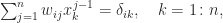
 is the Kronecker delta (equal to
  and
and  takes the value
  and
and  ,
,  . It is not hard to see that this polynomial is the Lagrange basis polynomial:
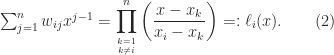

 denotes the sum of all distinct products of
  of the arguments
  (that is,
  is the
  and
and  has a checkerboard sign pattern: the
  .
.
 is a degree
 and
and  .
. and
and  :
:![\notag V = \left[\begin{array}{ccccc} 1 & 1 & 1 & 1 & 1\\ 0 & \frac{1}{4} & \frac{1}{2} & \frac{3}{4} & 1\\[\smallskipamount] 0 & \frac{1}{16} & \frac{1}{4} & \frac{9}{16} & 1\\[\smallskipamount] 0 & \frac{1}{64} & \frac{1}{8} & \frac{27}{64} & 1\\[\smallskipamount] 0 & \frac{1}{256} & \frac{1}{16} & \frac{81}{256} & 1 \end{array}\right], \quad V^{-1} = \left[\begin{array}{ccccc} 1 & -\frac{25}{3} & \frac{70}{3} & -\frac{80}{3} & \frac{32}{3}\\[\smallskipamount] 0 & 16 & -\frac{208}{3} & 96 & -\frac{128}{3}\\ 0 & -12 & 76 & -128 & 64\\[\smallskipamount] 0 & \frac{16}{3} & -\frac{112}{3} & \frac{224}{3} & -\frac{128}{3}\\[\smallskipamount] 0 & -1 & \frac{22}{3} & -16 & \frac{32}{3} \end{array}\right],](https://s0.wp.com/latex.php?latex=%5Cnotag+V+%3D+%5Cleft%5B%5Cbegin%7Barray%7D%7Bccccc%7D+1+%26+1+%26+1+%26+1+%26+1%5C%5C+0+%26+%5Cfrac%7B1%7D%7B4%7D+%26+%5Cfrac%7B1%7D%7B2%7D+%26+%5Cfrac%7B3%7D%7B4%7D+%26+1%5C%5C%5B%5Csmallskipamount%5D+0+%26+%5Cfrac%7B1%7D%7B16%7D+%26+%5Cfrac%7B1%7D%7B4%7D+%26+%5Cfrac%7B9%7D%7B16%7D+%26+1%5C%5C%5B%5Csmallskipamount%5D+0+%26+%5Cfrac%7B1%7D%7B64%7D+%26+%5Cfrac%7B1%7D%7B8%7D+%26+%5Cfrac%7B27%7D%7B64%7D+%26+1%5C%5C%5B%5Csmallskipamount%5D+0+%26+%5Cfrac%7B1%7D%7B256%7D+%26+%5Cfrac%7B1%7D%7B16%7D+%26+%5Cfrac%7B81%7D%7B256%7D+%26+1+%5Cend%7Barray%7D%5Cright%5D%2C+%5Cquad+V%5E%7B-1%7D+%3D+%5Cleft%5B%5Cbegin%7Barray%7D%7Bccccc%7D+1+%26+-%5Cfrac%7B25%7D%7B3%7D+%26+%5Cfrac%7B70%7D%7B3%7D+%26+-%5Cfrac%7B80%7D%7B3%7D+%26+%5Cfrac%7B32%7D%7B3%7D%5C%5C%5B%5Csmallskipamount%5D+0+%26+16+%26+-%5Cfrac%7B208%7D%7B3%7D+%26+96+%26+-%5Cfrac%7B128%7D%7B3%7D%5C%5C+0+%26+-12+%26+76+%26+-128+%26+64%5C%5C%5B%5Csmallskipamount%5D+0+%26+%5Cfrac%7B16%7D%7B3%7D+%26+-%5Cfrac%7B112%7D%7B3%7D+%26+%5Cfrac%7B224%7D%7B3%7D+%26+-%5Cfrac%7B128%7D%7B3%7D%5C%5C%5B%5Csmallskipamount%5D+0+%26+-1+%26+%5Cfrac%7B22%7D%7B3%7D+%26+-16+%26+%5Cfrac%7B32%7D%7B3%7D+%5Cend%7Barray%7D%5Cright%5D%2C+&bg=ffffff&fg=222222&s=0&c=20201002)
 .
. satisfies
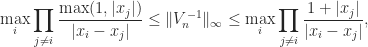
 for all
  (in particular, when
  for all
  . It is also known that for any set of real points
 we have
  , where the lower bound is an extremely fast growing function of the dimension!
 operation algorithm for solving
  of Björck and Pereyra (1970). There is now a long list of generalizations of this algorithm in various directions, including for confluent Vandermonde-like matrices (Higham, 1990), as well as for more specialized problems (Demmel and Koev, 2005) and more general ones (Bella et al., 2009). Another important observation is that the exponential lower bounds are for real nodes. For complex nodes
  can be much better conditioned. Indeed when the
  is the unitary Fourier matrix and so
  we obtain
 in the case of (4)).
 with
with  having degree
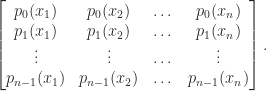
 , for any matrix norm, where
  is the spectral radius (the largest magnitude of any eigenvalue of
 ), but it can be arbitrarily weak for nonnormal matrices.
 , where the
  are the singular values of
  are of similar order of magnitude.
 ,
,  .
. matrices with
  , generated by
  the formula (3) is prone to overflow, which can be avoided by evaluating it in higher precision arithmetic.
 ,
,  of
of  . We can rewrite this upper bound as
 larger than (4), this factor being attained for
  .
. then (4) reduces to
 , where
 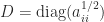 and
and  (thus
(thus  is a correlation matrix), using
 using (6). For example, for the
  Pascal matrix
![\notag P_5 = \left[\begin{array}{ccccc} 1 & 1 & 1 & 1 & 1\\ 1 & 2 & 3 & 4 & 5\\ 1 & 3 & 6 & 10 & 15\\ 1 & 4 & 10 & 20 & 35\\ 1 & 5 & 15 & 35 & 70 \end{array}\right]](https://s0.wp.com/latex.php?latex=%5Cnotag+P_5+%3D+%5Cleft%5B%5Cbegin%7Barray%7D%7Bccccc%7D+1+%26+1+%26+1+%26+1+%26+1%5C%5C+1+%26+2+%26+3+%26+4+%26+5%5C%5C+1+%26+3+%26+6+%26+10+%26+15%5C%5C+1+%26+4+%26+10+%26+20+%26+35%5C%5C+1+%26+5+%26+15+%26+35+%26+70+%5Cend%7Barray%7D%5Cright%5D+&bg=ffffff&fg=222222&s=0&c=20201002)
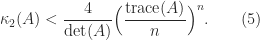
 . The bounds from (4) and (5) are both
  , whereas combining (4) and (7) gives a bound of
  .
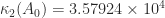
. for a matrix with integer entries. If a Cholesky, LU, or QR factorization of
  symmetric matrices with integer elements bounded by
  ; see
; see 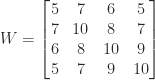
 . This little matrix has been used as an example and for test purposes in many research papers and books over the years, in particular by John Todd, who described it as “the notorious matrix
  of T. S. Wilson”.
 for a “positive definite symmetric
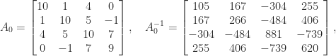
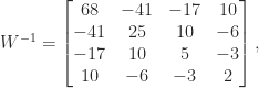
 . The matrix
  is therefore a factor 12 more ill conditioned than
 and found that about 0.21 percent of them had a larger condition number than
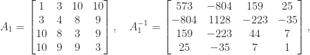
 . How far is this matrix from being a worst case?
 . It is possible to obtain a bound from first principles by using the relation
  , where
  ,
,
 , using the fact that
  is monotonically increasing for
  , gives
 ,
,
 , since
  we have
  , and hence
 . The bounds (1) and (2) remain valid if we modify the definitions of
  to allow zero elements (note that Rutishauser’s matrix
  elements. Exhaustively searching over the sets in reasonable time is possible with a carefully optimized code. Higham and Lettington (2021) use a MATLAB code that loops over all symmetric matrices with integer elements between
  (since
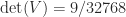
 . and determinant
  . The maximum over
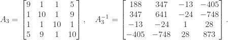
 and determinant


![\notag R = \begin{bmatrix} \sqrt{5} & \frac{7\,\sqrt{5}}{5} & \frac{6\,\sqrt{5}}{5} & \sqrt{5}\\[\smallskipamount] 0 & \frac{\sqrt{5}}{5} & -\frac{2\,\sqrt{5}}{5} & 0\\[\smallskipamount] 0 & 0 & \sqrt{2} & \frac{3\,\sqrt{2}}{2}\\[\smallskipamount] 0 & 0 & 0 & \frac{\sqrt{2}}{2} \end{bmatrix} \quad (W = R^TR).](https://s0.wp.com/latex.php?latex=%5Cnotag+R+%3D+%5Cbegin%7Bbmatrix%7D+%5Csqrt%7B5%7D+%26+%5Cfrac%7B7%5C%2C%5Csqrt%7B5%7D%7D%7B5%7D+%26+%5Cfrac%7B6%5C%2C%5Csqrt%7B5%7D%7D%7B5%7D+%26+%5Csqrt%7B5%7D%5C%5C%5B%5Csmallskipamount%5D+0+%26+%5Cfrac%7B%5Csqrt%7B5%7D%7D%7B5%7D+%26+-%5Cfrac%7B2%5C%2C%5Csqrt%7B5%7D%7D%7B5%7D+%26+0%5C%5C%5B%5Csmallskipamount%5D+0+%26+0+%26+%5Csqrt%7B2%7D+%26+%5Cfrac%7B3%5C%2C%5Csqrt%7B2%7D%7D%7B2%7D%5C%5C%5B%5Csmallskipamount%5D+0+%26+0+%26+0+%26+%5Cfrac%7B%5Csqrt%7B2%7D%7D%7B2%7D+%5Cend%7Bbmatrix%7D+%5Cquad+%28W+%3D+R%5ETR%29.+&bg=ffffff&fg=222222&s=0&c=20201002)
 element, it is unremarkable. If we factor out the diagonal then we obtain the
  factorization, which has rational elements:
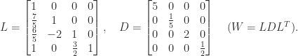
 with a
  matrix
  of integers. It is known that every symmetric positive definite
  with
with  , but examples are known for
  for which the factorization does not exist. This result is mentioned by Taussky (1961) and goes back to Hermite, Minkowski, and Mordell. Higham and Lettington (2021) found the integer factor
 it is necessary that a certain quadratic equation in
 and two rational factors:
![\notag Z_1=\left[ \begin{array}{cccc} \frac{1}{2} & 1 & 0 & 1 \\ \frac{3}{2} & 2 & 3 & 3 \\ \frac{1}{2} & 1 & 0 & 0 \\ \frac{3}{2} & 2 & 1 & 0 \\ \end{array} \right], \quad Z_2=\left[ \begin{array}{@{\mskip2mu}rrrr} \frac{3}{2} & 2 & 2 & 2 \\ \frac{3}{2} & 2 & 2 & 1 \\ \frac{1}{2} & 1 & 1 & 2 \\ -\frac{1}{2} & -1 & 1 & 1 \\ \end{array} \right].](https://s0.wp.com/latex.php?latex=%5Cnotag+Z_1%3D%5Cleft%5B+%5Cbegin%7Barray%7D%7Bcccc%7D++%5Cfrac%7B1%7D%7B2%7D+%26+1+%26+0+%26+1+%5C%5C++%5Cfrac%7B3%7D%7B2%7D+%26+2+%26+3+%26+3+%5C%5C++%5Cfrac%7B1%7D%7B2%7D+%26+1+%26+0+%26+0+%5C%5C++%5Cfrac%7B3%7D%7B2%7D+%26+2+%26+1+%26+0+%5C%5C+%5Cend%7Barray%7D+%5Cright%5D%2C+%5Cquad+Z_2%3D%5Cleft%5B+%5Cbegin%7Barray%7D%7B%40%7B%5Cmskip2mu%7Drrrr%7D++%5Cfrac%7B3%7D%7B2%7D+%26+2+%26+2+%26+2+%5C%5C++%5Cfrac%7B3%7D%7B2%7D+%26+2+%26+2+%26+1+%5C%5C++%5Cfrac%7B1%7D%7B2%7D+%26+1+%26+1+%26+2+%5C%5C++-%5Cfrac%7B1%7D%7B2%7D+%26+-1+%26+1+%26+1+%5C%5C+%5Cend%7Barray%7D+%5Cright%5D.+&bg=ffffff&fg=222222&s=0&c=20201002)
 of
of  (a problem also considered in Higham, Lettington, and Schmidt (2021)), with integer