Six matrix factorizations dominate in numerical linear algebra and matrix analysis: for most purposes one of them is sufficient for the task at hand. We summarize them here.
For each factorization we give the cost in flops for the standard method of computation, stating only the highest order terms. We also state the main uses of each factorization.
For full generality we state factorizations for complex matrices. Everything translates to the real case with “Hermitian” and “unitary” replaced by “symmetric” and “orthogonal”, respectively.
The terms “factorization” and “decomposition” are synonymous and it is a matter of convention which is used. Our list comprises three factorization and three decompositions.
Recall that an upper triangular matrix is a matrix of the form

and a lower triangular matrix is the transpose of an upper triangular one.
Cholesky Factorization
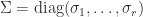
Every Hermitian positive definite matrix 


Cost: 
Use: solving positive definite linear systems.
LU Factorization
Any matrix 


Cost: 
Use: solving general linear systems.
QR Factorization
Any matrix 


![R = \left[\begin{smallmatrix} R_1 \\ 0\end{smallmatrix}\right]](https://s0.wp.com/latex.php?latex=R+%3D+%5Cleft%5B%5Cbegin%7Bsmallmatrix%7D+R_1+%5C%5C+0%5Cend%7Bsmallmatrix%7D%5Cright%5D&bg=ffffff&fg=222222&s=0&c=20201002)

Partitioning ![Q = [Q_1~Q_2]](https://s0.wp.com/latex.php?latex=Q+%3D+%5BQ_1%7EQ_2%5D&bg=ffffff&fg=222222&s=0&c=20201002)


Cost: 


Use: solving least squares problems, computing an orthonormal basis for the range space of
Schur Decomposition
Any matrix 


For real matrices, a special form of this decomposition exists in which all the factors are real. An upper quasi-triangular matrix 


Cost: 

Use: computing eigenvalues and eigenvectors, computing invariant subspaces, evaluating matrix functions.
Spectral Decomposition
Every Hermitian matrix 


Cost: 


Use: any problem involving eigenvalues of Hermitian matrices.
Singular Value Decomposition
Any matrix

where 


Cost: 


Use: determining matrix rank, solving rank-deficient least squares problems, computing all kinds of subspace information.
Discussion
Pivoting can be incorporated into both Cholesky factorization and QR factorization, giving 


The big six factorizations can all be computed by numerically stable algorithms. Another important factorization is that provided by the Jordan canonical form, but while it is a useful theoretical tool it cannot in general be computed in a numerically stable way.
For further details of these factorizations see the articles below.
These factorizations are precisely those discussed by Stewart (2000) in his article The Decompositional Approach to Matrix Computation, which explains the benefits of matrix factorizations in numerical linear algebra.
 of
of  is an invariant subspace of
  for all
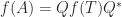
  . If we partition
 ![\notag A [Q_1,~Q_2] = [Q_1,~Q_2] \begin{bmatrix} T_{11} & T_{12} \\ 0 & T_{22} \\ \end{bmatrix},](https://s0.wp.com/latex.php?latex=%5Cnotag+++A+%5BQ_1%2C%7EQ_2%5D+%3D+%5BQ_1%2C%7EQ_2%5D+++%5Cbegin%7Bbmatrix%7D+++T_%7B11%7D+%26+T_%7B12%7D+%5C%5C+++++++0++%26+T_%7B22%7D+%5C%5C+++%5Cend%7Bbmatrix%7D%2C+&bg=ffffff&fg=222222&s=0&c=20201002)
 , showing that the columns of
  span an invariant subspace of
  . The first column of
  , but the other columns are not eigenvectors, in general. Eigenvectors can be computed by solving upper triangular systems involving
  , where
  is an eigenvalue.
 , where
  and
and  is strictly upper triangular. Taking Frobenius norms gives
 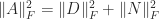 , or
, or
 is independent of the particular Schur decomposition and it provides a measure of the departure from normality. The matrix
  ) if and only if
  . So a normal matrix is unitarily diagonalizable:
  .
. shows that computing
  reduces to computing a function of a triangular matrix. Matrix functions illustrate what Van Loan (1975) describes as “one of the most basic tenets of numerical algebra”, namely “anything that the Jordan decomposition can do, the Schur decomposition can do better!”. Indeed the Jordan canonical form is built on a possibly ill conditioned similarity transformation while the Schur decomposition employs a perfectly conditioned unitary similarity, and the full upper triangular factor of the Schur form can do most of what the Jordan form’s bidiagonal factor can do.
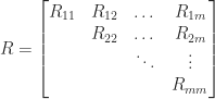
 has a real Schur decomposition
  in which in which all the factors are real,
  blocks
 ![R_{ii} = \left[\begin{array}{@{}rr@{\mskip2mu}} a & b \\ -b & a \end{array}\right], \quad b \ne 0,](https://s0.wp.com/latex.php?latex=R_%7Bii%7D+%3D+%5Cleft%5B%5Cbegin%7Barray%7D%7B%40%7B%7Drr%40%7B%5Cmskip2mu%7D%7D+a+%26+b+%5C%5C++++++++++++++++-b+%26+a+%5Cend%7Barray%7D%5Cright%5D%2C+%5Cquad+b+%5Cne+0%2C+&bg=ffffff&fg=222222&s=0&c=20201002)
 .
.