A Vandermonde matrix is defined in terms of scalars 


The 


Vandermonde matrices arise in polynomial interpolation. Suppose we wish to find a polynomial 


where ![a = [a_1,a_2,\dots,a_n]^T](https://s0.wp.com/latex.php?latex=a+%3D+%5Ba_1%2Ca_2%2C%5Cdots%2Ca_n%5D%5ET&bg=ffffff&fg=222222&s=0&c=20201002)

The problem

is called the primal problem, and it arises when we determine the weights for a quadrature rule: given moments 


Determinant
The determinant of 


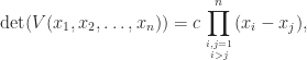
where, since both sides have degree 


This formula confirms that
Inverse
Now assume that 

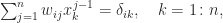
where 


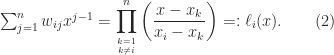
We deduce that

where 


From (1) and (3) we see that if the 


Note that summing (2) over
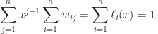
where the second equality follows from the fact that 

so the elements in the 

Example
To illustrate the formulas above, here is an example, with 

![\notag V = \left[\begin{array}{ccccc} 1 & 1 & 1 & 1 & 1\\ 0 & \frac{1}{4} & \frac{1}{2} & \frac{3}{4} & 1\\[\smallskipamount] 0 & \frac{1}{16} & \frac{1}{4} & \frac{9}{16} & 1\\[\smallskipamount] 0 & \frac{1}{64} & \frac{1}{8} & \frac{27}{64} & 1\\[\smallskipamount] 0 & \frac{1}{256} & \frac{1}{16} & \frac{81}{256} & 1 \end{array}\right], \quad V^{-1} = \left[\begin{array}{ccccc} 1 & -\frac{25}{3} & \frac{70}{3} & -\frac{80}{3} & \frac{32}{3}\\[\smallskipamount] 0 & 16 & -\frac{208}{3} & 96 & -\frac{128}{3}\\ 0 & -12 & 76 & -128 & 64\\[\smallskipamount] 0 & \frac{16}{3} & -\frac{112}{3} & \frac{224}{3} & -\frac{128}{3}\\[\smallskipamount] 0 & -1 & \frac{22}{3} & -16 & \frac{32}{3} \end{array}\right],](https://s0.wp.com/latex.php?latex=%5Cnotag+V+%3D+%5Cleft%5B%5Cbegin%7Barray%7D%7Bccccc%7D+1+%26+1+%26+1+%26+1+%26+1%5C%5C+0+%26+%5Cfrac%7B1%7D%7B4%7D+%26+%5Cfrac%7B1%7D%7B2%7D+%26+%5Cfrac%7B3%7D%7B4%7D+%26+1%5C%5C%5B%5Csmallskipamount%5D+0+%26+%5Cfrac%7B1%7D%7B16%7D+%26+%5Cfrac%7B1%7D%7B4%7D+%26+%5Cfrac%7B9%7D%7B16%7D+%26+1%5C%5C%5B%5Csmallskipamount%5D+0+%26+%5Cfrac%7B1%7D%7B64%7D+%26+%5Cfrac%7B1%7D%7B8%7D+%26+%5Cfrac%7B27%7D%7B64%7D+%26+1%5C%5C%5B%5Csmallskipamount%5D+0+%26+%5Cfrac%7B1%7D%7B256%7D+%26+%5Cfrac%7B1%7D%7B16%7D+%26+%5Cfrac%7B81%7D%7B256%7D+%26+1+%5Cend%7Barray%7D%5Cright%5D%2C+%5Cquad+V%5E%7B-1%7D+%3D+%5Cleft%5B%5Cbegin%7Barray%7D%7Bccccc%7D+1+%26+-%5Cfrac%7B25%7D%7B3%7D+%26+%5Cfrac%7B70%7D%7B3%7D+%26+-%5Cfrac%7B80%7D%7B3%7D+%26+%5Cfrac%7B32%7D%7B3%7D%5C%5C%5B%5Csmallskipamount%5D+0+%26+16+%26+-%5Cfrac%7B208%7D%7B3%7D+%26+96+%26+-%5Cfrac%7B128%7D%7B3%7D%5C%5C+0+%26+-12+%26+76+%26+-128+%26+64%5C%5C%5B%5Csmallskipamount%5D+0+%26+%5Cfrac%7B16%7D%7B3%7D+%26+-%5Cfrac%7B112%7D%7B3%7D+%26+%5Cfrac%7B224%7D%7B3%7D+%26+-%5Cfrac%7B128%7D%7B3%7D%5C%5C%5B%5Csmallskipamount%5D+0+%26+-1+%26+%5Cfrac%7B22%7D%7B3%7D+%26+-16+%26+%5Cfrac%7B32%7D%7B3%7D+%5Cend%7Barray%7D%5Cright%5D%2C+&bg=ffffff&fg=222222&s=0&c=20201002)
for which 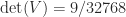
Conditioning
Vandermonde matrices are notorious for being ill conditioned. The ill conditioning stems from the monomials being a poor basis for the polynomials on the real line. For arbitrary distinct points 
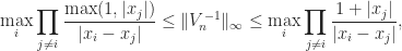
with equality on the right when 


and that for 

These exponential lower bounds are alarming, but they do not necessarily rule out the use of Vandermonde matrices in practice. One of the reasons is that there are specialized algorithms for solving Vandermonde systems whose accuracy is not dependent on the condition number 


Generalizations
Two ways in which Vandermonde matrices have been generalized are by allowing confluency of the points 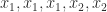

The transpose of a confluent Vandermonde matrix arises in Hermite interpolation; it is nonsingular if the points corresponding to the “nonconfluent columns” are distinct (that is, if 
A Vandermonde-like matrix is defined in terms of a set of polynomials 

Of most interest are polynomials that satisfy a three-term recurrence, in particular, orthogonal polynomials. Such matrices can be much better conditioned than general Vandermonde matrices.
Notes
Algorithms for solving confluent Vandermonde-like systems and their rounding error analysis are described in the chapter “Vandermonde systems” of Higham (2002).
Gautschi has written many papers on the conditioning of Vandermonde matrices, beginning in 1962. We mention just his most recent paper on this topic: Gautschi (2011).
References
This is a minimal set of references, which contain further useful references within.
- T. Bella, Y. Eidelman. I. Gohberg. I. Koltracht, and V. Olshevsky, A Fast Björck–Pereyra-Type Algorithm for Solving Hessenberg-Quasiseparable-Vandermonde Systems, SIAM J. Matrix Anal. Appl. 31(2), 790–815, 2009.
- James W. Demmel and Plamen Koev, The Accurate and Efficient Solution of a Totally Positive Generalized Vandermonde Linear System, SIAM J. Matrix Anal. Appl. 2791, 142–152, 2005.
- Walter Gautschi, Optimally Scaled and Optimally Conditioned Vandermonde and Vandermonde-like matrices, BIT 51, 103–125, 2011.
- Nicholas J. Higham, Accuracy and Stability of Numerical Algorithms, second edition, Society for Industrial and Applied Mathematics, Philadelphia, PA, USA, 2002.
- Nicholas J. Higham, Stability Analysis of Algorithms for Solving Confluent Vandermonde-like Systems, SIAM J. Matrix Anal. Appl. 11, 23–41, 1990.
Related Blog Posts
- What Is a Condition Number? (2020)
This article is part of the “What Is” series, available from https://nhigham.com/category/what-is and in PDF form from the GitHub repository https://github.com/higham/what-is.

A few interesting tidbits regarding Vandermonde matrices.
Since det V has a nice closed form Vandermonde systems are one of the few places where one can meaningfully apply Cramer’s rule.
If a set of nodes maximize |det V| they are known as Fekete points. In one dimension the Fekete points are the Gauss-Legendre-Lobatto nodes (GLL); a result which I believe was first shown by Fejér. The proof is tedious. A cottage industry exists around trying to find Fekete points in higher dimensional domains with applications to multi-variate Lagrange interpolation.