What Is the Hilbert Matrix?

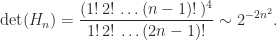
The Hilbert matrix $H_n = (h_{ij})$ is the $n\times n$ matrix with $h_{ij} = 1/(i+j-1)$ . For example,

$H_4 = \left[\begin{array}{@{\mskip 5mu}c*{3}{@{\mskip 15mu} c}@{\mskip 5mu}} 1 & \frac{1}{2} & \frac{1}{3} & \frac{1}{4} \\[6pt] \frac{1}{2} & \frac{1}{3} & \frac{1}{4} & \frac{1}{5}\\[6pt] \frac{1}{3} & \frac{1}{4} & \frac{1}{5} & \frac{1}{6}\\[6pt] \frac{1}{4} & \frac{1}{5} & \frac{1}{6} & \frac{1}{7}\\[6pt] \end{array}\right].$

It is probably the most famous test matrix and its conditioning and other properties were extensively studied in the early days of digital computing, especially by John Todd.

The Hilbert matrix is symmetric and it is a Hankel matrix (constant along the anti-diagonals). Less obviously, it is symmetric positive definite (all its eigenvalues are positive) and totally positive (every submatrix has positive determinant). Its condition number grows rapidly with $n$ ; indeed for the 2-norm the asymptotic growth rate is $\kappa_2(H_n) \sim \mathrm{e}^{3.5n}$ . An underlying reason for the ill conditioning is that the Hilbert matrix is obtained when least squares polynomial approximation is done using the monomial basis, and this is known to be an ill-conditioned polynomial basis.

The inverse of $H_n$ has integer entries, with $(i,j)$ entry

$(-1)^{i+j} (i+j-1) \displaystyle{ n+i-1 \choose n-j } { n+j-1 \choose n-i } { i+j-2 \choose i-1 }^2.$

For example,

$H_4^{-1} = \left[\begin{array}{rrrr} 16 & -120 & 240 & -140 \\ -120 & 1200 & -2700 & 1680 \\ 240 & -2700 & 6480 & -4200 \\ -140 & 1680 & -4200 & 2800 \\ \end{array}\right].$

The alternating sign pattern is a consequence of total positivity.

The determinant is also known explicitly:

$\det(H_n) = \displaystyle\frac{ (1!\, 2!\, \dots (n-1)!\, )^4 }{ 1!\, 2!\, \dots (2n-1)! } \sim 2^{-2n^2}. % \cite{todd54}$

The Hilbert matrix is infinitely divisible, which means that the matrix with $(i,j)$ element $h_{ij}^t$ is positive semidefinite for all nonnegative real numbers $t$ .

Other interesting matrices can be formed from the Hilbert matrix. The Lotkin matrix, A = gallery('lotkin',n) in MATLAB, is the Hilbert matrix with the first row replaced by $1$ s, making it nonsymmetric. Like the Hilbert matrix, it is ill conditioned and has an inverse with integer entries. For the $n\times n$ matrix with $(i,j)$ entry $1/(i+j)$ , which is a submatrix of $H_{n+1}$ , the largest singular value tends to $\pi$ as $n\to\infty$ , with error decaying slowly as $O(1/\log n)$ , as was shown by Taussky.

The Hilbert matrix is not a good test matrix, for several reasons. First, it is too ill conditioned, being numerically singular in IEEE double precision arithmetic for $n = 12$ . Second, it is too special: the definiteness and total positivity, together with the fact that it is a special case of a Cauchy matrix (which has elements $1/(x_i + y_j)$ ), mean that certain quantities associated with it can be calculated more accurately than for a general positive definite matrix. The third reason why the Hilbert matrix is not a good test matrix is that most of its elements cannot be stored exactly in floating-point arithmetic, so the matrix actually stored is a perturbation of $H_n$ —and since $H_n$ is ill conditioned this means (for example) that the inverse of the stored matrix can be very different from the exact inverse. A way around this might be to work the integer matrix $H_n^{-1}$ , but its elements are exactly representable in double precision only for $n\le 12$ .

MATLAB has functions hilb and invhilb for the Hilbert matrix and its inverse. How to efficiently form the Hilbert matrix in MATLAB is an interesting question. The hilb function essentially uses the code

j = 1:n;
H = 1./(j'+j-1)

This code is more concise and efficient than two nested loops would be. The second line may appear to be syntactically incorrect, because j'+j adds a column vector to a row vector. However, the MATLAB implicit expansion feature expands j' into an $n\times n$ matrix in which every column is j', expands j into an $n\times n$ matrix in which every row is j, then adds the two matrices. It is not hard to see that the Hilbert matrix is the result of these two lines of code.

References

This is a minimal set of references, which contain further useful references within.

Rajendra Bhatia, Infinitely divisible matrices, Amer. Math. Monthly 113(3), 221–235, 2006.
Man-Duen Choi, Tricks or treats with the Hilbert matrix, Amer. Math. Monthly 90(5), 301–312, 1983
Nicholas J. Higham, Accuracy and Stability of Numerical Algorithms, second edition, Society for Industrial and Applied Mathematics, Philadelphia, PA, USA, 2002. Section 28.1.
M. Lotkin, A set of test matrices, M.T.A.C. 9(52), 153–161, 1955.

What Is a Fréchet Derivative?

Let $U$ and $V$ be Banach spaces (complete normed vector spaces). The Fréchet derivative of a function $f:U \to V$ at $X\in U$ is a linear mapping $L:U\to V$ such that

$\notag f(X+E) - f(X) - L(X,E) = o(\|E\|)$

for all $E\in U$ . The notation $L(X,E)$ should be read as “the Fréchet derivative of $f$ at $X$ in the direction $E$ ”. The Fréchet derivative may not exist, but if it does exist then it is unique. When $U = V = \mathbb{R}$ , the Fréchet derivative is just the usual derivative of a scalar function: $L(x,e) = f'(x)e$ .

As a simple example, consider $U = V = \mathbb{R}^{n\times n}$ and $f(X) = X^2$ . From the expansion

$f(X+E) - f(X) = XE + EX + E^2$

we deduce that $L(X,E) = XE + EX$ , the first order part of the expansion. If $X$ commutes with $E$ then $L_X(E) = 2XE = 2EX$ .

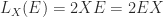More generally, it can be shown that if $f$ has the power series expansion $f(x) = \sum_{i=0}^\infty a_i x^i$ with radius of convergence $r$ then for $X,E\in\mathbb{R}^{n\times n}$ with $\|X\| < r$ , the Fréchet derivative is

$L(X,E) = \displaystyle\sum_{i=1}^\infty a_i \displaystyle\sum_{j=1}^i X^{j-1} E X^{i-j}.$

An explicit formula for the Fréchet derivative of the matrix exponential, $f(A) = \mathrm{e}^A$ , is

$L(A,E) = \displaystyle\int_0^1 \mathrm{e}^{A(1-s)} E \mathrm{e}^{As} \, ds.$

Like the scalar derivative, the Fréchet derivative satisfies sum and product rules: if $g$ and $h$ are Fréchet differentiable at $A$ then

$\notag \begin{alignedat}{2} f &= \alpha g + \beta h &&\;\Rightarrow\; L_f(A,E) = \alpha L_g(A,E) + \beta L_h(A,E),\\ f &= gh &&\;\Rightarrow\; L_f(A,E) = L_g(A,E) h(A) + g(A) L_h(A,E). \end{alignedat}$

A key requirement of the definition of Fréchet derivative is that $L(X,E)$ must satisfy the defining equation for all $E$ . This is what makes the Fréchet derivative different from the Gâteaux derivative (or directional derivative), which is the mapping $G:U \to V$ given by

$\notag G(X,E) = \lim_{t\to0} \displaystyle\frac{f(X+t E)-f(X)}{t} = \frac{\mathrm{d}}{\mathrm{dt}}\Bigm|_{t=0} f(X + tE).$

Here, the limit only needs to exist in the particular direction $E$ . If the Fréchet derivative exists at $X$ then it is equal to the Gâteaux derivative, but the converse is not true.

A natural definition of condition number of $f$ is

$\mathrm{cond}(f,X) = \lim_{\epsilon\to0} \displaystyle\sup_{\|\Delta X\| \le \epsilon \|X\|} \displaystyle\frac{\|f(X+\Delta X) - f(X)\|}{\epsilon\|f(X)\|},$

and it can be shown that $\mathrm{cond}$ is given in terms of the Fréchet derivative by

$\mathrm{cond}(f,X) = \displaystyle\frac{\|L(X)\| \|X\|}{\|f(X)\|},$

where

$\|L(X)\| = \sup_{Z\ne0}\displaystyle\frac{\|L(X,Z)\|}{\|Z\|}.$

For matrix functions, the Fréchet derivative has a number of interesting properties, one of which is that the eigenvalues of $L(X)$ are the divided differences

$\notag f[\lambda_i,\lambda_j] = \begin{cases} \dfrac{ f(\lambda_i)-f(\lambda_j) }{\lambda_i - \lambda_j}, & \lambda_i\ne\lambda_j, \\ f'(\lambda_i), & \lambda_i=\lambda_j, \end{cases}$

for $1\le i,j \le n$ , where the $\lambda_i$ are the eigenvalues of $X$ . We can check this formula in the case $F(X) = X^2$ . Let $(\lambda,u)$ be an eigenpair of $X$ and $(\mu,v)$ an eigenpair of $X^T$ , so that $Xu = \lambda u$ and $X^Tv = \mu v$ , and let $E = uv^T$ . Then

$L(X,E) = XE + EX = Xuv^T + uv^TX = (\lambda + \mu) uv^T.$

So $uv^T$ is an eigenvector of $L(X)$ with eigenvalue $\lambda + \mu$ . But $f[\lambda,\mu] = (\lambda^2-\mu^2)/(\lambda - \mu) = \lambda + \mu$ (whether or not $\lambda$ and $\mu$ are distinct).

References

This is a minimal set of references, which contain further useful references within.

Kendall Atkinson and Weimin Han, Theoretical Numerical Analysis: A Functional Analysis Framework, Springer-Verlag, New York, 2009. (Section 5.3).
Nicholas J. Higham, Functions of Matrices: Theory and Computation, Society for Industrial and Applied Mathematics, Philadelphia, PA, USA, 2008. (Chapter 3).
James Ortega and Werner Rheinboldt, Iterative Solution of Nonlinear Equations in Several Variables, Society for Industrial and Applied Mathematics, Philadelphia, PA, 2000. (Section 3.1).

Six Useful LaTeX Packages

Here are six $\LaTeX$ packages that, while they are perhaps not among the best known, I have found to be very useful. All of them are probably available in your $\LaTeX$ distribution, but in case they are not I give links to the packages on CTAN (the Comprehensive TeX Archive Network). A PDF file containing a demonstration of the examples below is available here.

Mathtools

Mathtools extends the amsmath package with various additions, particularly for fine-tuning the typesetting of equations, and it also fixes a few problems with amsmath. To give just one example, the standard amsmath bmatrix environment centres its columns:

A = \begin{bmatrix}
     12 & 3  & 0 \\
     0  & 10 &-1 
   \end{bmatrix}

For matrices with negative elements, such as this one, the columns can look better right justified. The bmatrix* environment provided by mathtools allows a column alignment parameter to be given, so we can right justify the columns as follows:

A = \begin{bmatrix*}[r]
     12 & 3  & 0 \\
     0  & 10 &-1 
   \end{bmatrix*}

Unfortunately, only one alignment parameter can be given, so this command does not allow different columns to have different alignments (to achieve this, we can use the array environment instead).

The mathtools package is regularly updated.

Url

The url package provides the \url command, which acts like \verb except that it allows line breaks to be made when the argument is typeset. I use url whenever I need to typeset a URL or a path, in particular in my BibTeX bib files. I call the package with the hyphens option, so that line breaks will be allowed at hyphens. Example:

\usepackage[hyphens]{url}
...
\footnote{\url{https://icl.bitbucket.io/hpl-ai/}}
\url{http://blogs.mathworks.com/cleve/2013/01/07/george-forsythe/}

An advantage over the \verb command is that \url (or, if necessary, \urldef) can be used inside another command, such as \footnote, as in this example.

Upref

By loading the upref package you ensure that every \ref or \eqref reference is set in an upright font. This is normal typesetting practice, but it is not enforced by all $\LaTeX$ classes. It is enforced by the SIAM class, for example.

Siunitx

The siunitx package typesets SI units according to the official rules, with just the right spacing between the number and the unit. For example, you can type

\si{kg.m/s^2}

instead of

$\mathrm{kg}\,\mathrm{m}/\mathrm{s}^2$

Even if you do not need to type SI units, you might find useful the package’s ability to round and format numbers.

Upquote

The upquote package forces left and right quotes to be typed as straight (vertical) quotes in \verb and verbatim environments. This is usually what is required in program listings. We used upquote in MATLAB Guide.

Fancyvrb

The fancyvrb package provides a more powerful replacement for the verbatim environment, allowing the font to be specified, the environment to be boxed, an external file to be inclued in a verbatim environment, and much more. Here is example that formats the contents of the environment in blue and boldface:

\begin{Verbatim}[fontsize=\small,formatcom=\color{blue}]
>> syms x, int(1/(1-x^4))
ans =
atan(x)/2 + atanh(x)/2
\end{Verbatim}

The second example includes an external file, numbers the lines, and puts horizontal lines before and after the code:

\renewcommand{\theFancyVerbLine}%
{\textcolor{red}{\small\arabic{FancyVerbLine}}}
\VerbatimInput[frame=lines,numbers=left,fontsize=\small]%
{d:/matlab/gen/gf.m}

Other packages

I have previously written about the enumitem and booktabs packages, which I also strongly recommend.

What Is the Adjugate of a Matrix?

The adjugate of an $n\times n$ matrix $A$ is defined by

$\mathrm{adj}(A) = \bigl( (-1)^{i+j} \det(A_{ji}) \bigr),$

where $A_{pq}$ denotes the submatrix of $A$ obtained by deleting row $p$ and column $q$ . It is the transposed matrix of cofactors. The adjugate is sometimes called the (classical) adjoint and is sometimes written as $A^\mathrm{A}$ .

The adjugate satisfies

$A \mathrm{adj}(A) = \mathrm{adj}(A) A = \det(A)I,$

so for nonsingular $A$ ,

$\mathrm{adj}(A) = \det(A) A^{-1},$

and this equation is often used to give a formula for $A^{-1}$ in terms of determinants.

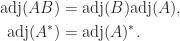
Since the adjugate is a scalar multiple of the inverse, we would expect it to share some properties of the inverse. Indeed we have

$\begin{aligned} \mathrm{adj}(AB) &= \mathrm{adj}(B) \mathrm{adj}(A),\\ \mathrm{adj}(A^*) &= \mathrm{adj}(A)^*. \end{aligned}$

These properties can be proved by first assuming the matrices are nonsingular—in which case they follow from properties of the determinant and the inverse—and then using continuity of the entries of $\mathrm{adj}(A)$ and the fact that every matrix is the limit of a sequence of nonsingular matrices. Another property that can be proved in a similar way is

$\mathrm{adj}\bigl(\mathrm{adj}(A)\bigr) = (\det A)^{n-2} A.$

If $A$ has rank $n-2$ or less then $\mathrm{adj}(A)$ is just the zero matrix. Indeed in this case every $(n-1)\times(n-1)$ submatrix of $A$ is singular, so $\det(A_{ji}) \equiv 0$ in the definition of $\mathrm{adj}(A)$ . In particular, $\mathrm{adj}(0) = 0$ and $\mathrm{adj}(xy^*) = 0$ for any rank-1 matrix $xy^*$

Less obviously, if $\mathrm{rank}(A) = n-1$ then $\mathrm{adj}(A)$ has rank 1. This can be seen from the formula below that expresses the adjugate in terms of the singular value decomposition (SVD).

If $x,y\in\mathbb{C}^n$ , then for nonsingular $A$ ,

$\begin{aligned} \det(A + xy^*) &= \det\bigl( A(I + A^{-1}x y^*) \bigr)\\ &= \det(A) \det( I + A^{-1}x y^*)\\ &= \det(A) (1+ y^*A^{-1}x)\\ &= \det(A) + y^* (\det(A)A^{-1})x\\ &= \det(A) + y^* \mathrm{adj}(A)x. \end{aligned}$

Again it follows by continuity that for any $A$ ,

$\det(A + xy^*) = \det(A) + y^* \mathrm{adj}(A)x.$

This expression is useful when we need to deal with a rank-1 perturbation to a singular matrix. A related identity is

$\det\left( \begin{bmatrix} A & x \\ y^* & \alpha \\ \end{bmatrix}\right) = \alpha \det(A) - y^* \mathrm{adj}(A) x.$

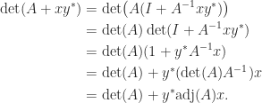
Let $A = U\Sigma V^*$ be an SVD, where $U$ and $V$ are unitary and $\Sigma = \mathrm{diag}(\sigma_i)$ , with $\sigma_1 \ge \sigma_2 \ge \cdots \ge \sigma_n \ge 0$ . Then

$\mathrm{adj}(A) = \mathrm{adj}(V^*) \mathrm{adj}(\Sigma) \mathrm{adj}(U) = \mathrm{adj}(V)^* \mathrm{adj}(\Sigma) \mathrm{adj}(U).$

It is easy to see that $D = \mathrm{adj}(\Sigma)$ is diagonal, with

$d_{kk} = \displaystyle\prod_{i=1\atop i\ne k }^n \sigma_i.$

Since $U$ and $V$ are unitary and hence nonsingular,

$\begin{aligned} \mathrm{adj}(A) &= \mathrm{adj}(V)^* \mathrm{adj}(\Sigma) \mathrm{adj}(U)\\ &= \overline{\det(V)} V^{-*} \mathrm{adj}(\Sigma) \det(U) U^{-1}\\ &= \overline{\det(V)} V \mathrm{adj}(\Sigma) \det(U) U^*\\ &= \overline{\det(V)} \det(U) \cdot V \mathrm{adj}(\Sigma) U^*. \end{aligned}$

If $\mathrm{rank}(A) = n-1$ then $\sigma_n = 0$ and so

$\mathrm{adj}(A) = \rho\, \sigma_1 \sigma_2 \cdots \sigma_{n-1}v_n^{} u_n^*,$

where $\rho = \overline{\det(V)} \det(U)$ has modulus $1$ and $v_n$ and $u_n$ are the last columns of $V$ and $U$ , respectively.

The definition of $\mathrm{adj}(A)$ does not provide a good means for computing it, because the determinant computations are prohibitively expensive. The following MATLAB function (which is very similar to the function adjoint in the Symbolic Math Toolbox) uses the SVD formula.

function X = adj(A)
%ADJ     Adjugate of a matrix.
%   X = ADJ(A) computes the adjugate of the square matrix A via
%   the singular value decomposition.

n = length(A);
[U,S,V] = svd(A);
D = zeros(n);
for i=1:n
    d = diag(S);
    d(i) = 1;
    D(i,i) = prod(d);
end
X = conj(det(V))*det(U)*V*D*U';

Note that, in common with most SVD codes, the svd function does not return $\det(U)$ and $\det(V)$ , so we must compute them. This function is numerically stable, as shown by Stewart (1998).

Finally, we note that Richter (1954) and Mirsky (1956) obtained the Frobenius norm bound

$\|\mathrm{adj}(A) \|_F \le \displaystyle\frac{ \|A\|_F^{n-1} }{ n^{(n-2)/2} }.$

References

This is a minimal set of references, which contain further useful references within.

Roger A. Horn and Charles R. Johnson, Matrix Analysis, second edition, Cambridge University Press, 2013. Section 0.8.2.
L. Mirsky, The Norms of Adjugate and Inverse Matrices, Archiv der Mathematik 7(4), 276–277, 1956.
Hans Richter, Bemerkung zur Norm der Inversen einer Matrix, Archiv der Mathematik 5, 447–448, 1954.
G. W. Stewart, On the Adjugate Matrix, Linear Algebra Appl. 283, 151–164, 1998.

This article is part of the “What Is” series, available from https://nhigham.com/category/what-is and in PDF form from the GitHub repository https://github.com/higham/what-is.

Update (August 10, 2020): added the second displayed equation.

What Is a Matrix Function?

If you give an array as the argument to a mathematical function in a programming language or problem solving environment you are likely to receive the result of applying the function to each component of the array. For example, here MATLAB exponentiates the integers from 0 to 3:

>> A = [0 1; 2 3], X = exp(A)
A =
    0     1
    2     3
X =
   1.0000e+00   2.7183e+00
   7.3891e+00   2.0086e+01

When the array represents a matrix this componentwise evaluation is not useful, as it does not obey the rules of matrix algebra. To see what properties we might require, consider the matrix square root. This function is notable historically because Cayley considered it in the 1858 paper in which he introduced matrix algebra.

A square root of an $n\times n$ matrix $A$ is a matrix $X$ such that $X^2 = A$ . Any square root $X$ satisfies

$AX = X^2 X = X X^2 = XA,$

so $X$ commutes with $A$ . Also, $A^* = (X^2)^* = (X^*)^2$ , so $X^*$ is a square root of $A^*$ (here, the superscript $*$ denotes the conjugate transpose).

Furthermore, for any nonsingular matrix $Z$ we have

$(Z^{-1}XZ)^2 = Z^{-1}X^2 Z = Z^{-1}A Z.$

If we choose $Z$ as a matrix that takes $A$ to its Jordan canonical form $J$ then we have $(Z^{-1}XZ)^2 = J$ , so that $Z^{-1}XZ$ is a square root of $J$ , or in other words $X$ can be expressed as $X = Z \sqrt{J} Z^{-1}$ .

Generalizing from these properties of the matrix square root it is reasonable to ask that a function $f(A)$ of a square matrix $A$ satisfies

$f(A)$ commutes with $A$ ,
$f(A^*) = f(A)^*$ ,
$f(A) = Z f(J)Z^{-1}$ , where $A$ has the Jordan canonical form $A = ZJZ^{-1}$ .

(These are of course not the only requirements; indeed $f(A) \equiv I$ satisfies all three conditions.)

Many definitions of $f(A)$ can be given that satisfy these and other natural conditions. We will describe just three definitions (a notable omission is a definition in terms of polynomial interpolation).

Power Series

For a function $f$ that has a power series expansion we can define $f(A)$ by substituting $A$ for the variable. It can be shown that the matrix series will be convergent for matrices whose eigenvalues lie within the radius of convergence of the scalar power series. For example, where $\rho$ denotes the spectral radius. This definition is natural for functions that have a power series expansion, but it is rather limited in its applicability.

$\begin{aligned} \cos(A) &= I - \displaystyle\frac{A^2}{2!} + \frac{A^4}{4!} - \frac{A^6}{6!} + \cdots,\\ \log(I+A) &= A - \displaystyle\frac{A^2}{2} + \frac{A^3}{3} - \frac{A^4}{4} + \cdots, \quad \rho(A)<1, \end{aligned}$

Jordan Canonical Form Definition

If $A$ has the Jordan canonical form

$Z^{-1}AZ = J = \mathrm{diag}(J_1, J_2, \dots, J_p),$

where

$J_k = J_k(\lambda_k) = \begin{bmatrix} \lambda_k & 1 & & \\ & \lambda_k & \ddots & \\ & & \ddots & 1 \\ & & & \lambda_k \end{bmatrix} = \lambda_k I + N \in \mathbb{C}^{m_k\times m_k},$

then

$f(A) := Z f(J) Z^{-1} = Z \mathrm{diag}(f(J_k)) Z^{-1},$

where

$f(J_k) := \begin{bmatrix} f(\lambda_k) & f'(\lambda_k) & \dots & \displaystyle\frac{f^{(m_k-1)}(\lambda_k)}{(m_k-1)!} \\ & f(\lambda_k) & \ddots & \vdots \\ & & \ddots & f'(\lambda_k) \\ & & & f(\lambda_k) \end{bmatrix}.$

Notice that $f(J_k)$ has the derivatives of $f$ along its diagonals in the upper triangle. Write $J_k = \lambda_k I + N$ , where $N$ is zero apart from a superdiagonal of 1s. The formula for $f(J_k)$ is just the Taylor series expansion

$f(J_k) = f(\lambda_k I + N) = f(\lambda_k)I + f'(\lambda_k)N + \displaystyle\frac{f''(\lambda_k)}{2!}N^2 + \cdots + \displaystyle\frac{f^{(m_k-1)}(\lambda_k)}{(m_k-1)!}N^{m_k-1}.$

The series is finite because $N^{m_k} = 0$ : as $N$ is powered up the superdiagonal of 1s moves towards the right-hand corner until it eventually disappears.

An immediate consequence of this formula is that $f(A)$ is defined only if the necessary derivatives exist: for each eigenvalue $\lambda_k$ we need the existence of the derivatives at $\lambda_k$ of order up to one less than the size of the largest Jordan block in which $\lambda_k$ appears.

When $A$ is a diagonalizable matrix the definition simplifies considerably: if $A = ZDZ^{-1}$ with $D = \mathrm{diag}(\lambda_i)$ then $f(A) = Zf(D)Z^{-1} = Z \mathrm{diag}(\lambda_i) Z^{-1}$ .

Cauchy Integral Formula

For a function $f$ analytic on and inside a closed contour $\Gamma$ that encloses the spectrum of $A$ the matrix $f(A)$ can be defined by the Cauchy integral formula

$f(A) := \displaystyle\frac{1}{2\pi \mathrm{i}} \int_\Gamma f(z) (zI-A)^{-1} \,\mathrm{d}z.$

This formula is mathematically elegant and can be used to provide short proofs of certain theoretical results.

Equivalence of Definitions

These and several other definitions turn out to be equivalent under suitable conditions. This was recognized by Rinehart, who wrote in 1955

“There have been proposed in the literature since 1880 eight distinct definitions of a matric function, by Weyr, Sylvester and Buchheim, Giorgi, Cartan, Fantappiè, Cipolla, Schwerdtfeger and Richter … All of the definitions except those of Weyr and Cipolla are essentially equivalent.”

Computing a Matrix Function in MATLAB

In MATLAB, matrix functions are distinguished from componentwise array evaluation by the postfix “m” on a function name. Thus expm, logm, and sqrtm are matrix function counterparts of exp, log, and sqrt. Compare the example at the start of this article with

>> A = [0 1; 2 3], X = expm(A)
A =
    0     1
    2     3
X =
   5.2892e+00   8.4033e+00
   1.6807e+01   3.0499e+01

The MATLAB function funm calculates $f(A)$ for general matrix functions $f$ (subject to some restrictions).

References

This is a minimal set of references, which contain further useful references within.

Nicholas J. Higham, Functions of Matrices: Theory and Computation, Society for Industrial and Applied Mathematics, Philadelphia, PA, USA, 2008.
Roger Horn and Charles Johnson, Topics in Matrix Analysis, Cambridge University Press, 1991.
R. F. Rinehart, The Equivalence of Definitions of a Matric Function, Amer. Math. Monthly 62(6), 395-414, 1955.

Randsvd Matrices with Large Growth Factors

Sixty years ago James Wilkinson published his backward error analysis of Gaussian elimination for solving a linear system $Ax = b$ , where $A$ is a nonsingular $n\times n$ matrix. He showed that in floating-point arithmetic the computed solution $\widehat{x}$ satisfies

$(A+\Delta A) \widehat{x} = b, \qquad \|\Delta A\|_{\infty} \le p(n) \rho_n u \|A\|_{\infty},$

where $u$ is the unit roundoff and $p$ is a low degree polynomial. The term $\rho_n$ is the growth factor, defined by

$\rho_n = \displaystyle\frac{\max_{i,j,k} |a_{ij}^{(k)}|} {\max_{i,j}|a_{ij}|} \ge 1,$

where the $a_{ij}^{(k)}$ are the elements at the $k$ th stage of Gaussian elimination. The growth factor measures how much elements grow during the elimination. We would like the product $p(n)\rho_n$ to be of order 1, so that $\Delta A$ is a small relative perturbation of $A$ . We therefore need $\rho_n$ not to be too large.

With partial pivoting, in which row interchanges are used to ensure that at each stage the pivot element is the largest in its column, Wilkinson showed that $\rho_n \le 2^{n-1}$ and that equality is possible. Such exponential growth implies a large $\Delta A$ (unless we are lucky), meaning a severe loss of numerical stability. However, seventy years of digital computing experience have shown that $\rho_n$ is usually of modest size in practice. Explaining why this is the case is one of the outstanding problems in numerical analysis.

It is easy to experiment with growth factors in MATLAB. I will use the function

function g = gf(A)
%GF     Approximate growth factor.
%   g = GF(A) is an approximation to the
%   growth factor for LU factorization
%   with partial pivoting.
[~,U] = lu(A);
g = max(abs(U),[],'all')/max(abs(A),[],'all');

It computes a lower bound on the growth factor (since it only considers $k=n$ in the numerator in the definition), but it is entirely adequate for our purposes here. Let’s compute the growth factor for a random matrix of order 10,000 with elements from the standard normal distribution (mean 0, variance 1):

>> rng(1); n = 10000; gf(randn(n))
ans =
6.1335e+01

Growth of 61 is unremarkable for a matrix of this size. Now we try a matrix of the same size generated by the gallery('randsvd') function:

>> A = gallery('randsvd',n,1e6,2,[],[],1);
>> gf(A)
ans =
9.7544e+02

This function generates an $n\times n$ matrix with known singular value distribution and with singular vector matrices that are random orthogonal matrices from the Haar distribution. The parameter 1e6 specifies the 2-norm condition number, while the 2 (the mode parameter) specifies that there is only one small singular value, so the singular values are 1 repeated $n-1$ times and 1e-6. Growth of 975 is exceptional! These matrices have been in MATLAB since the 1990s, but this large growth property has apparently not been noticed before.

It turns out that mode 2 randsvd matrices generate with high probability growth factors of size at least $n/(4 \log n)$ for any condition number and for any pivoting strategy, not just partial pivoting. One way to check this is to randomly permute the columns of $A$ before doing the LU factorization with partial pivoting:

>> gf(A(:,randperm(n)))
ans =
7.8395e+02

Here is a plot showing the maximum over 12 randsvd matrices for each $n$ of the growth factors for three different pivoting strategies, along with the maximum growth factors for partial pivoting for rand and randn matrices. The black curve is $n/(4 \log n)$ . This plot emphasizes the unusually large growth for mode 2 randsvd matrices.

What is the explanation for this large growth? It stems from three facts.

Haar distributed orthogonal matrices have the property that that their elements are fairly small with high probability, as shown by Jiang in 2005.
If the largest entries in magnitude of $A$ and $A^{-1}$ are both small, in the sense that their product is $\theta \ll 1$ , then $A$ will produce a growth factor of at least $1/\theta$ for any pivoting strategy. This was proved by Des Higham and I in the paper Large Growth Factors in Gaussian Elimination with Pivoting.
If $W$ is an orthogonal matrix generating large growth then a rank-1 perturbation of 2-norm at most 1 tends to preserve the large growth.

For full details see the new EPrint Random Matrices Generating Large Growth in LU Factorization with Pivoting by Des Higham, Srikara Pranesh and me.

Is growth of order $n$ a problem in practice? It can be for two reasons.

The largest dense linear systems $Ax = b$ solved today are of dimension $n = 10^7$ . If we work in single precision then $nu \approx 1$ and so LU factorization can potentially be completely unstable if there is growth of order $n$ .
For IEEE half precision arithmetic growth of order $n$ will cause overflow once $n$ exceeds $10^5 / \max_{i,j} |a_{ij}|$ . It was overflow in half precision LU factorization on randsvd matrices that alerted us to the large growth.

What Is Bfloat16 Arithmetic?

Bfloat16 is a floating-point number format proposed by Google. The name stands for “Brain Floating Point Format” and it originates from the Google Brain artificial intelligence research group at Google.

Bfloat16 is a 16-bit, base 2 storage format that allocates 8 bits for the significand and 8 bits for the exponent. It contrasts with the IEEE fp16 (half precision) format, which allocates 11 bits for the significand but only 5 bits for the exponent. In both cases the implicit leading bit of the significand is not stored, hence the “+1” in this diagram:

The motivation for bfloat16, with its large exponent range, was that “neural networks are far more sensitive to the size of the exponent than that of the mantissa” (Wang and Kanwar, 2019).

Bfloat16 uses the same number of bits for the exponent as the IEEE fp32 (single precision) format. This makes conversion between fp32 and bfloat16 easy (the exponent is kept unchanged and the significand is rounded or truncated from 24 bits to 8) and the possibility of overflow in the conversion is largely avoided. Overflow can still happen, though (depending on the rounding mode): the significand of fp32 is longer, so the largest fp32 number exceeds the largest bfloat16 number, as can be seen in the following table. Here, the precision of the arithmetic is measured by the unit roundoff, which is $2^{-t}$ , where $t$ is the number of bits in the significand.

Note that although the table shows the minimum positive subnormal number for bfloat16, current implementations of bfloat16 do not appear to support subnormal numbers (this is not always clear from the documentation).

As the unit roundoff values in the table show, bfloat16 numbers have the equivalent of about three decimal digits of precision, which is very low compared with the eight and sixteen digits, respectively, of fp32 and fp64 (double precision).

The next table gives the number of numbers in the bfloat16, fp16, and fp32 systems. It shows that the bfloat16 number system is very small compared with fp32, containing only about 65,000 numbers.

The spacing of the bfloat16 numbers is large far from 1. For example, 65280, 65536, and 66048 are three consecutive bfloat16 numbers.

At the time of writing, bfloat16 is available, or announced, on four platforms or architectures.

The Google Tensor Processing Units (TPUs, versions 2 and 3) use bfloat16 within the matrix multiplication units. In version 3 of the TPU the matrix multiplication units carry out the multiplication of 128-by-128 matrices.
The NVIDIA A100 GPU, based on the NVIDIA Ampere architecture, supports bfloat16 in its tensor cores through block fused multiply-adds (FMAs) $C + A*B$ with 8-by-8 $A$ and 8-by-4 $B$ .
Intel has published a specification for bfloat16 and how it intends to implement it in hardware. The specification includes an FMA unit that takes as input two bfloat16 numbers $a$ and $b$ and an fp32 number $c$ and computes $c + a*b$ at fp32 precision, returning an fp32 number.
The Arm A64 instruction set supports bfloat16. In particular, it includes a block FMA $C + A*B$ with 2-by-4 $A$ and 4-by-2 $B$ .

The pros and cons of bfloat16 arithmetic versus IEEE fp16 arithmetic are

bfloat16 has about one less (roughly three versus four) digit of equivalent decimal precision than fp16,
bfloat16 has a much wider range than fp16, and
current bfloat16 implementations do not support subnormal numbers, while fp16 does.

If you wish to experiment with bfloat16 but do not have access to hardware that supports it you will need to simulate it. In MATLAB this can be done with the chop function written by me and Srikara Pranesh.

References

This is a minimal set of references, which contain further useful references within.

Arm A64 Instruction Set Architecture Armv8, for Armv8-A Architecture Profile, ARM Limited, 2019.
Intel Corporation, BFLOAT16—Hardware Numerics Definition, 2018.
IEEE Standard for Floating-Point Arithmetic, IEEE Std 754-2019 (Revision of IEEE 754-2008), The Institute of Electrical and Electronics Engineers, New York, 2019.
NVIDIA Corporation, NVIDIA A100 Tensor Core GPU Architecture, 2020.

Month: June 2020

What Is the Hilbert Matrix?

References

Related Blog Posts

What Is a Fréchet Derivative?

References

Related Blog Posts

Six Useful LaTeX Packages

Mathtools

Url

Upref

Siunitx

Upquote

Fancyvrb

Other packages

What Is the Adjugate of a Matrix?

References

What Is a Matrix Function?

Power Series

Jordan Canonical Form Definition

Cauchy Integral Formula

Equivalence of Definitions

Computing a Matrix Function in MATLAB

References

Related Blog Posts

Randsvd Matrices with Large Growth Factors

What Is Bfloat16 Arithmetic?

References

Related Blog Posts

References

Related Blog Posts

Share this:

References

Related Blog Posts

Share this:

Mathtools

Url

Upref

Siunitx

Upquote

Fancyvrb

Other packages

Share this:

References

Share this:

Power Series

Jordan Canonical Form Definition

Cauchy Integral Formula

Equivalence of Definitions

Computing a Matrix Function in MATLAB

References

Related Blog Posts

Share this:

Share this:

References

Related Blog Posts

Share this: