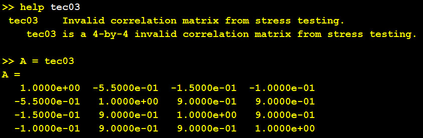
The Top 10 Algorithms in Applied Mathematics

From “Computational Science” by David E. Keyes in Princeton Companion to Applied Mathematics

In the January/February 2000 issue of Computing in Science and Engineering, Jack Dongarra and Francis Sullivan chose the “10 algorithms with the greatest influence on the development and practice of science and engineering in the 20th century” and presented a group of articles on them that they had commissioned and edited. (A SIAM News article by Barry Cipra gives a summary for anyone who does not have access to the original articles). This top ten list has attracted a lot of interest.

Sixteen years later, I though it would be interesting to produce such a list in a different way and see how it compares with the original top ten. My unscientific—but well defined— way of doing so is to determine which algorithms have the most page locators in the index of The Princeton Companion to Applied Mathematics (PCAM). This is a flawed measure for several reasons. First, the book focuses on applied mathematics, so some algorithms included in the original list may be outside its scope, though the book takes a broad view of the subject and includes many articles about applications and about topics on the interface with other areas. Second, the content is selective and the book does not attempt to cover all of applied mathematics. Third, the number of page locators is not necessarily a good measure of importance. However, the index was prepared by a professional indexer, so it should reflect the content of the book fairly objectively.

A problem facing anyone who compiles such a list is to define what is meant by “algorithm”. Where does one draw the line between an algorithm and a technique? For a simple example, is putting a rational function in partial fraction form an algorithm? In compiling the following list I have erred on the side of inclusion. This top ten list is in decreasing order of the number of page locators.

Newton and quasi-Newton methods
Matrix factorizations (LU, Cholesky, QR)
Singular value decomposition, QR and QZ algorithms
Monte-Carlo methods
Fast Fourier transform
Krylov subspace methods (conjugate gradients, Lanczos, GMRES, minres)
JPEG
PageRank
Simplex algorithm
Kalman filter

Note that JPEG (1992) and PageRank (1998) were youngsters in 2000, but all the other algorithms date back at least to the 1960s.

By comparison, the 2000 list is, in chronological order (no other ordering was given)

Metropolis algorithm for Monte Carlo
Simplex method for linear programming
Krylov subspace iteration methods
The decompositional approach to matrix computations
The Fortran optimizing compiler
QR algorithm for computing eigenvalues
Quicksort algorithm for sorting
Fast Fourier transform
Integer relation detection
Fast multipole method

The two lists agree in 7 of their entries. The differences are:

PCAM list	2000 list
Newton and quasi-Newton methods	The Fortran Optimizing Compiler
Jpeg	Quicksort algorithm for sorting
PageRank	Integer relation detection
Kalman filter	Fast multipole method

Of those in the right-hand column, Fortran is in the index of PCAM and would have made the list, but so would C, MATLAB, etc., and I draw the line at including languages and compilers; the fast multipole method nearly made the PCAM table; and quicksort and integer relation detection both have one page locator in the PCAM index.

There is a remarkable agreement between the two lists! Dongarra and Sullivan say they knew that “whatever we came up with in the end, it would be controversial”. Their top ten has certainly stimulated some debate, but I don’t think it has been too controversial. This comparison suggests that Dongarra and Sullivan did a pretty good job, and one that has stood the test of time well.

Finally, I point readers to a talk Who invented the great numerical algorithms? by Nick Trefethen for a historical perspective on algorithms, including most of those mentioned above.

A Collection of Invalid Correlation Matrices

I’ve written before (here) about the increasingly common problem of matrices that are supposed to be correlation matrices (symmetric and positive semidefinite with ones on the diagonal) turning out to have some negative eigenvalues. This is usually bad news because it means that subsequent computations are unjustified and even dangerous. The problem occurs in a wide variety of situations. For example in portfolio optimization a consequence could be to take arbitrarily large positions in a stock, as discussed by Schmelzer and Hauser in Seven Sins in Portfolio Optimization.

Much research has been done over the last fifteen years or so on how to compute the nearest correlation matrix to a given matrix, and these techniques provide a natural way to correct an “invalid” correlation matrix. Of course, other approaches can be used, such as going back to the underlying data and massaging it appropriately, but it is clear from the literature that this is not always possible and practitioners may not have the mathematical or statistical knowledge to do it.

Nataša Strabić and I have built up a collection of invalid correlation matrices, which we used most recently in work on Bounds for the Distance to the Nearest Correlation Matrix. These are mostly real-life matrices, which makes them valuable for test purposes.

We have made our collection of invalid correlation matrices available in MATLAB form on GitHub as the repository matrices-correlation-invalid. I am delighted to be able to include, with the permission of investment company Orbis, two relatively large matrices, of dimensions 1399 and 3120, arising in finance. These were the matrices I used in my original 2002 paper.

Behind the Scenes of the Princeton Companion to Applied Mathematics

I’ve published an article Making the Princeton Companion to Applied Mathematics in Mathematics Today, the membership magazine of the The Institute of Mathematics and its Applications.

The article describes the story behind the Princeton Companion to Applied Mathematics, published in October 2015, which I edited (along with associate editors Mark Dennis, Paul Glendinning, Paul Martin, Fadil Santosa and Jared Tanner).

Among the topics covered are

the motivation for the book and for publishing it in hard copy (as well as in e-book form),
the question “What is applied mathematics?”,
the challenge of producing 1000 pages of high quality typeset mathematical text,
the design of the book.

Complementary to the article is the YouTube video below, recorded and produced by George Miller, in which I talk about the project. It was filmed in and around the Alan Turing building at the University of Manchester. An interesting tidbit about George is that when he worked at Oxford University Press he set up and commissioned the Very Short Introductions series, of which Tim Gowers’s Mathematics: Very Short Introductions was one of the first volumes to be published.

Empty Matrices in MATLAB

What matrix has zero norm, unit determinant, and is its own inverse? The conventional answer would be that there is no such matrix. But the empty matrix [ ] in MATLAB satisfies these conditions:

>> A = []; norm(A), det(A), inv(A)
ans =
     0
ans =
     1
ans =
     []

While many MATLAB users will be familiar with the use of [ ] as a way of removing a row or column of a matrix (e.g., A(:,1) = []), or omitting an argument in a function call (e.g., max(A,[],2)), fewer will be aware that [ ] is just one in a whole family of empty matrices. Indeed [ ] is the 0-by-0 empty matrix

>> size([])
ans =
     0     0

Empty matrices can have dimension n-by-0 or 0-by-n for any nonnegative integer n. One way to construct them is with double.empty (or the empty method of any other MATLAB class):

>> double.empty
ans =
     []
>> double.empty(4,0)
ans =
   Empty matrix: 4-by-0

What makes empty matrices particularly useful is that they satisfy natural generalizations of the rules of matrix algebra. In particular, matrix multiplicaton is defined whenever the inner dimensions match up.

>> A = double.empty(0,5)*double.empty(5,0)
A =
     []
>> A = double.empty(2,0)*double.empty(0,4)
A =
     0     0     0     0
     0     0     0     0

As the second example shows, the product of empty matrices with positive outer dimensions has zero entries. This ensures that expressions like the following work as we would hope:

>> p = 0; A = ones(3,2); B = ones(3,p); C = ones(2,3); D = ones(p,3);
>> [A B]*[C; D]
ans =
     2     2     2
     2     2     2
     2     2     2

In examples such as this empty matrices are very convenient, as they avoid us having to program around edge cases.

Empty matrices have been in MATLAB since 1986, their inclusion having been suggested by Rod Smart and Rob Schreiber $\lbrack 1 \rbrack$ . A 1989 MATLAB manual says

We’re not sure we’ve done it correctly, or even consistently, but we have found the idea useful.

In those days there was only one empty matrix, the 0-by-0 matrix, and this led Nett and Haddad (1993) to describe the MATLAB implementation of the empty matrix concept as “neither correct, consistent, or useful, at least not for system-theoretic applications”. Nowadays MATLAB gets it right and indeed it adheres to the rules suggested by those authors and by de Boor (1990). If you are wondering how the values for norm([]), det([]) and inv([]) given above are obtained, see de Boor’s article for an explanation in terms of linear algebra transformations.

The concept of empty matrices dates back to before MATLAB. The earliest reference I am aware of is a 1970 book by Stoer and Witzgall. As the extract below shows, these authors recognized the need to support empty matrices of varying dimension and they understood how multiplication of empty matrices should work.

Reference

John N. Little, The MathWorks Newsletter, 1 (1), March 1986.

Updated Catalogue of Software for Matrix Functions

Edvin Deadman and I have updated the catalogue of software for matrix functions that we produced in 2014 (and which was discussed in this post). The new version, which has undergone some minor reorganization, is available here. It covers what is available in languages (C++, Fortran, Java, Julia, Python), problem solving environments (GNU Octave, Maple, Mathematica, MATLAB, R, Scilab), and libraries (GNU Scientific Library, NAG Library, SLICOT).

Here are some highlights of changes in the last two years that are reflected in the new version.

MATLAB functions expm and logm have been improved.
Several new MATLAB third-party functions have been written, by various authors.
The NAG Library Mark 25 has been released, which includes many new codes for matrix functions.
Matrix function support in Julia has improved.

Other changes to the catalogue include these.

SLICOT has been added.
Two more R packages are included.

Suggestions for inclusion in a future revision are welcome.

The Improved MATLAB Functions Expm and Logm

Equation from the Princeton Companion to Applied Mathematics, article “Functions of Matrices” (p. 97)

The matrix exponential is a ubiquitous matrix function, important both for theory and for practical computation. The matrix logarithm, an inverse to the exponential, is also increasingly used (see my earlier post, 400 Years of Logarithms).

MATLAB R2015b introduced new versions of the expm and logm functions. The Release Notes say

The algorithms for expm, logm, and sqrtm show increased accuracy, with logm and sqrtm additionally showing improved performance.

The help text for expm and logm is essentially unchanged from the previous versions, so what’s different about the new functions? (I will discuss sqrtm in a future post.)

The answer is that both functions make use of new backward error bounds that can be much smaller than the old ones for very nonnormal matrices, and so help to avoid a phenomenon known as overscaling. The key change is that when bounding a matrix power series $p(X) = a_0 I + a_1 X + a_2 X^2 + \cdots$ , instead of bounding the $k$ th term $a_k X^k$ by $|a_k| \|X\|^k$ , a potentially smaller bound is used.

This is best illustrated by example. Suppose we want to bound $\|X^{12}\|$ and are not willing to compute $X^{12}$ but are willing to compute lower powers of $X$ . We have $12 = 6 \times 2 = 4 \times 3$ , so $\|X^{12}\|$ is bounded by each of the terms $(\|X^2\|)^6$ , $(\|X^3\|)^4$ , $(\|X^4\|)^3$ , and $(\|X^6\|)^2$ . 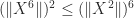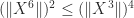But it is easy to see that $(\|X^6\|)^2 \le (\|X^2\|)^6$ and $(\|X^6\|)^2 \le (\|X^3\|)^4$ , so we can discard two of the bounds, ending up with

$\|X^{12}\| \le \min( \|X^4\|^3, \|X^6\|^2 ).$

This argument can be generalized so that every power of $X$ is bounded in terms of the norms of $X^p$ for values of $p$ up to some small, fixed value. The gains can be significant. Consider the matrix

$X = \begin{bmatrix}1 & 100 \\ 0 & 1 \end{bmatrix}.$

We have $\|X\|^{12} \approx 10^{24}$ , but

$X^k = \begin{bmatrix}1 & 100k \\ 0 & 1 \end{bmatrix},$

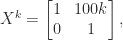
so the bound above is roughly $\|X^{12}\| \le 6 \times 10^{7}$ , which is a significant improvement.

One way to understand what is happening is to note the inequality

$\rho(X) \le \| X^k\| ^{1/k} \le \|X\|,$

where $\rho$ is the spectral radius (the largest modulus of any eigenvalue). The upper bound corresponds to the usual analysis. The lower bound is something that we cannot use to bound the norm of the power series. The middle term is what we are using, and as $k\to\infty$ the middle term converges to the lower bound, which can be arbitrarily smaller than the upper bound.

What is the effect of these bounds on the algorithms in expm and logm? Both algorithms make use of Padé approximants, which are good only for small-normed matrices, so the algorithms begin by reducing the norm of the input matrix. Backward error bounds derived by bounding a power series as above guide the norm reduction and if the bounds are weak then the norm is reduced too much, which can result in loss of accuracy in floating point arithmetic—the phenomenon of overscaling. The new bounds greatly reduce the chance of overscaling.

In his blog post A Balancing Act for the Matrix Exponential, Cleve Moler describes a badly scaled 3-by-3 matrix for which the original expm suffers from overscaling and a loss of accuracy, but notes that the new algorithm does an excellent job.

The new logm has another fundamental change: it applies inverse scaling and squaring and Padé approximation to the whole triangular Schur factor, whereas the previous logm applied this technique to the individual diagonal blocks in conjunction with the Parlett recurrence.

For more on the algorithms underlying the new codes see these papers. The details of how the norm of a matrix power series is bounded are given in Section 4 of the first paper.

A. H. Al-Mohy and N. J. Higham. A new scaling and squaring algorithm for the matrix exponential, SIAM J. Matrix Anal. Appl. 31(3), 970–989, 2009.
A. H. Al-Mohy and N. J. Higham. Improved inverse scaling and squaring algorithms for the matrix logarithm, SIAM J. Sci. Comp. 34(4), 153–169, 2012.
A. H. Al-Mohy, N. J. Higham and S. D. Relton. Computing the Fréchet derivative of the matrix logarithm and estimating the condition number, SIAM J. Sci. Comp. 35(4), 394–410, 2013.

Share this:

Share this:

Share this:

Reference

Share this:

Share this:

Share this: