In linear algebra terms, a correlation matrix is a symmetric positive semidefinite matrix with unit diagonal. In other words, it is a symmetric matrix with ones on the diagonal whose eigenvalues are all nonnegative.
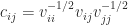
The term comes from statistics. If 


where 


where 

Here are a few facts.
- The elements of a correlation matrix lie on the interval
.
- The eigenvalues of a correlation matrix lie on the interval
.
- The eigenvalues of a correlation matrix sum to
(since the eigenvalues of a matrix sum to its trace).
- The maximal possible determinant of a correlation matrix is
.
It is usually not easy to tell whether a given matrix is a correlation matrix. For example, the matrix

is not a correlation matrix: it has eigenvalues 


A particularly simple class of correlation matrices is the one-parameter class 


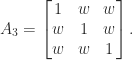
The matrix 
In some applications it is required to generate random correlation matrices, for example in Monte-Carlo simulations in finance. A method for generating random correlation matrices with a specified eigenvalue distribution was proposed by Bendel and Mickey (1978); Davies and Higham (2000) give improvements to the method. This method is implemented in the MATLAB function gallery('randcorr').
Obtaining or estimating correlations can be difficult in practice. In finance, market data is often missing or stale; different assets may be sampled at different time points (e.g., some daily and others weekly); and the matrices may be generated from different parametrized models that are not consistent. Similar problems arise in many other applications. As a result, correlation matrices obtained in practice may not be positive semidefinite, which can lead to undesirable consequences such as an investment portfolio with negative risk.
In risk management and insurance, matrix entries may be estimated, prescribed by regulations or assigned by expert judgement, but some entries may be unknown.
Two problems therefore commonly arise in connection with correlation matrices.
Nearest Correlation Matrix
Here, we have an approximate correlation matrix 

We may also have a requirement that certain elements of 
Another variation requires 
Another approach that can be used for restoring definiteness, although it does not in general produce the nearest correlation matrix, is shrinking, which constructs a convex linear combination 

Correlation Matrix Completion
Here, we have a partially specified matrix and we wish to complete it, that is, fill in the missing elements in order to obtain a correlation matrix. It is known that a completion is possible for any set of specified entries if the associate graph is chordal (Grone et al., 1994). In general, if there is one completion there are many, but there is a unique one of maximal determinant, which is elegantly characterized by the property that the inverse contains zeros in the positions of the unspecified entries.
References
This is a minimal set of references, and they cite further useful references.
- Rüdiger Borsdorf, Nicholas J. Higham and Marcos Raydan, Computing a nearest correlation matrix with factor structure, SIAM J. Matrix Anal. Appl. 31(5), 2603–2622, 2010
- Rüdiger Borsdorf and Nicholas J. Higham, A preconditioned Newton algorithm for the nearest correlation matrix, J. Numer. Anal. 30(1), 94–107, 2010.
- Philip I. Davies and Nicholas J. Higham, Numerically stable generation of correlation matrices and their factors, BIT 40(4), 640–651, 2000
- Dan I. Georgescu, Nicholas J. Higham and Gareth W. Peters, Explicit solutions to correlation matrix completion problems, with an application to risk management and insurance, Roy. Soc. Open Sci. 5(3), 1–11, 2018.
- Robert Grone, Charles R. Johnson, Eduardo M. Sá and Henry Wolkowicz, Positive definite completions of partial Hermitian matrices, Linear Algebra Appl. 58, 109–124, 1984.
- Nicholas J. Higham, Computing the nearest correlation matrix—A problem from finance, IMAJNA J. Numer. Anal. 22(3), 329–343, 2002.
- Houduo Qi and Defeng Sun, A quadratically convergent Newton method for computing the nearest correlation matrix, SIAM J. Matrix Anal. Appl. 28(2), 360–385, 2006
- Nicholas J. Higham, Nataša Strabić and Vedran Šego, Restoring definiteness via shrinking, with an application to correlation matrices with a fixed block, SIAM Rev. 58(2), 245–263, 2016.
- Numerical Algorithms Group, Nearest Correlation Matrix, 2019.
Related Blog Posts
- The Nearest Correlation Matrix, 2013.
- Anderson Acceleration, 2015.
- A Collection of Invalid Correlation Matrices, 2016.
- Completing Correlation Matrices (with D. I. Georgescu), Bank Underground, 2018.
