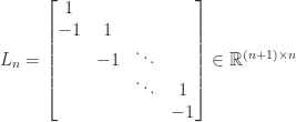
What Is the Second Difference Matrix?

The second difference matrix is the tridiagonal matrix $T_n$ with diagonal elements $2$ and sub- and superdiagonal elements $-1$ :

$\notag T_n = \left[ \begin{array}{@{}*{4}{r@{\mskip10mu}}r} 2 & -1 & & & \\ -1 & 2 & -1 & & \\[-5pt] & -1 & 2 & \ddots & \\ & & \ddots & \ddots & -1 \\ & & & -1 & 2 \end{array}\right] \in\mathbb{R}^{n\times n}.$

It arises when a second derivative is approximated by the central second difference $f''(x) \approx (f(x+h) -2 f(x) + f(x-h))/h^2$ . (Accordingly, the second difference matrix is sometimes defined as $-T_n$ .) In MATLAB, $T_n$ can be generated by gallery('tridiag',n), which is returned as a aparse matrix.

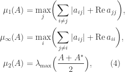
This is Gil Strang’s favorite matrix. The photo, from his home page, shows a birthday cake representation of the matrix.

The second difference matrix is symmetric positive definite. The easiest way to see this is to define the full rank rectangular matrix

$\notag L_n = \begin{bmatrix} 1 & & & \\ -1 & 1 & & \\ & -1 & \ddots & \\ & & \ddots & 1 \\ & & & -1 \end{bmatrix} \in\mathbb{R}^{(n+1)\times n}$

and note that $T_n = L_n^T L_n$ . The factorization corresponds to representing a central difference as the product of a forward difference and a backward difference. Other properties of the second difference matrix are that it is diagonally dominant, a Toeplitz matrix, and an $M$ -matrix.

Cholesky Factorization

In an LU factorization $A = LU$ the pivots $u_{ii}$ are $2$ , $3/2$ , $4/3$ , …, $(n+1)/n$ . Hence the pivots form a decreasing sequence tending to 1 as $n\to\infty$ . The diagonal of the Cholesky factor contains the square roots of the pivots. This means that in the Cholesky factorization $A = R^*R$ with $R$ upper bidiagonal, $r_{nn} \to 1$ and $r_{n,n-1}\to -1$ as $n\to\infty$ .

Determinant, Inverse, Condition Number

Since the determinant is the product of the pivots, $\det(T_n) = n+1$ .

The inverse of $T_n$ is full, with $(i,j)$ element $i(n-j+1)/(n+1)$ for $j\ge i$ . For example,

$\notag T_5^{-1} = \displaystyle\frac{1}{6} \begin{bmatrix} 5 & 4 & 3 & 2 & 1\\ 4 & 8 & 6 & 4 & 2\\ 3 & 6 & 9 & 6 & 3\\ 2 & 4 & 6 & 8 & 4\\ 1 & 2 & 3 & 4 & 5 \end{bmatrix}.$

The $2$ -norm condition number satisfies $\kappa_2(T_n) \sim 4n^2/\pi^2$ (as follows from the formula (1) below for the eigenvalues).

Eigenvalues and Eigenvectors

The eigenvalues of $T_n$ are

$\notag \mu_k = 4 \sin^2\Bigl(\displaystyle\frac{k \phi}{2} \Bigr), \quad k = 1:n, \qquad (1)$

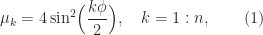
where $\phi = \pi/(n+1)$ , with corresponding eigenvector

$\notag v_k = \begin{bmatrix} \sin(k\phi), &\sin(2k\phi), &\dots, &\sin(nk\phi) \end{bmatrix}^T.$

The matrix $Q$ with

$\notag q_{ij} = \Bigl(\displaystyle\frac{2}{n+1}\Bigr)^{1/2} \sin\Bigl( \frac{ij\pi}{n+1} \Bigr)$

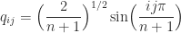
is therefore an eigenvector matrix for $T_n$ : $Q^*AQ = \mathrm{diag}(\mu_k)$ .

Variations

Various modifications of the second difference matrix arise and similar results can be derived. For example, consider the matrix obtained by changing the $(n,n)$ element to $1$ :

$\notag \widetilde{T}_n = \left[ \begin{array}{@{}*{4}{r@{\mskip10mu}}r} 2 & -1 & & & \\ -1 & 2 & -1 & & \\[-5pt] & -1 & 2 & \ddots & \\ & & \ddots & \ddots & -1 \\ & & & -1 & 1 \end{array}\right] \in\mathbb{R}^{n\times n}.$

It can be shown that $\widetilde{T}_n^{-1}$ has $(i,j)$ element $\min(i,j)$ and eigenvalues $4\cos( j \pi/(2n+1))^2$ , $j=1:n$ .

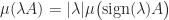
If we perturb the $(1,1)$ of $\widetilde{T}_n$ to $1$ , we obtain a singular matrix, but suppose we perturb the $(1,1)$ element to $3$ :

$\notag \widehat{T}_n = \left[ \begin{array}{@{}*{4}{r@{\mskip10mu}}r} 3 & -1 & & & \\ -1 & 2 & -1 & & \\[-5pt] & -1 & 2 & \ddots & \\ & & \ddots & \ddots & -1 \\ & & & -1 & 1 \end{array}\right] \in\mathbb{R}^{n\times n}.$

The inverse is $\widehat{T}_n^{-1} = G/2$ , where $G$ with $(i,j)$ element $2\min(i,j)-1$ is a matrix of Givens, and the eigenvalues are $4\cos((2j-1)\pi/(4n))^2$ , $j=1:n$ .

Notes

The factorization $T_n = L_n^TL_n$ is noted by Strang (2012).

For a derivation of the eigenvalues and eigenvectors see Todd (1977, p. 155 ff.). For the eigenvalues of $\widetilde{T}_n$ see Fortiana and Cuadras (1997). Givens’s matrix is described by Newman and Todd (1958) and Todd (1977).

References

This is a minimal set of references, which contain further useful references within.

J. Fortiana and C. N. Cuadras, A Family of Matrices, the Discretized Brownian Bridge, and Distance-Based Regression, Linear Algebra Appl. 264, 173–188, 1997.
Morris Newman and John Todd, The Evaluation of Matrix Inversion Programs, J. Soc. Indust. Appl. Math. 6(4), 466–476, 1958.
Gilbert Strang, Essays in Linear Algebra, Wellesley-Cambridge Press, Wellesley, MA, USA, 2012. Chapter A.3: “My Favorite Matrix”.
John Todd, Basic Numerical Mathematics, Vol. $2$ : Numerical Algebra, Birkhäuser, Basel, and Academic Press, New York, 1977.

What Is the Frank Matrix?

The $n\times n$ upper Hessenberg matrix

$\notag F_n = \left[\begin{array}{*{6}c} n & n-1 & n-2 & \dots & 2 & 1 \\ n-1 & n-1 & n-2 & \dots & 2 & 1 \\ 0 & n-2 & n-2 & \dots & 2 & 1 \\[-3pt] \vdots & 0 & \ddots & \ddots & \vdots & 1 \\[-3pt] \vdots & \vdots & \dots & 2 & 2 & 1 \\ 0 & 0 & \dots & 0 & 1 & 1 \\ \end{array}\right]$

was introduced by Frank in 1958 as a test matrix for eigensolvers.

Determinant

Taking the Laplace expansion about the first column, we obtain $\det(F_n) = n\det(F_{n-1}) - (n-1)\det(F_{n-1}) = \det(F_{n-1})$ , and since $\det(F_1) = 1$ we have $\det(F_n) = 1$ .

In MATLAB, the computed determinant of the matrix and its transpose can be far from the exact values of $1$ :

>> n = 20; F = anymatrix('gallery/frank',n); 
>> [det(F), det(F')]
ans =
   1.0000e+00  -1.4320e+01
>> n = 49; F = anymatrix('gallery/frank',n); det(F)
ans =
    -1.406934439401568e+45

This behavior illustrates the sensitivity of the determinant rather than numerical instability in the evaluation and it is very dependent on the arithmetic (different results may be obtained in different releases of MATLAB). The sensitivity can be seen by noting that

$\notag \det\bigl(F_n + \epsilon e_1e_n^T\bigr) = 1 + (-1)^{n-1} (n-1)!\epsilon, \qquad (1)$

which means that changing the $(1,n)$ element from 1 to $1+\epsilon$ changes the determinant by $(n-1)!\epsilon$ .

Inverse and Condition Number

It is easily verified that

$\notag F_n = \begin{bmatrix} 1 & -1 & & & \\ & 1 & -1 & & \\ & & 1 & \ddots & \\ & & & \ddots & -1\\ & & & & 1 \end{bmatrix}^{-1} \begin{bmatrix} 1 & & & & \\ n-1 & 1 & & & \\ & n-2& 1 & & \\ & & \ddots& \ddots & \\ & & & 1 & 1 \end{bmatrix} \equiv U^{-1}L. \qquad (2)$

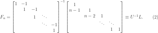
Hence $F_n^{-1} = L^{-1}U$ is lower Hessenberg with integer entries. This factorization provides another way to see that $\det(F_n) = 1$ .

From (1) we see that $F_n + \epsilon e_1e_n^T$ is singular for $\epsilon = (-1)^n/(n-1)!$ , which implies that

$\notag \kappa(F_n) \ge (n-1)! \|F_n\|$

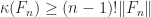
for any subordinate matrix norm, showing that the condition number grows very rapidly with $n$ . In fact, this lower bound is within a factor $3.5$ of the condition number for the $1$ -, $2$ -, and $\infty$ -norms for $n\le 20$ .

Eigenvalues

Denote by $p_n(t) = \det(F_n - tI)$ the characteristic polynomial of $F_n$ . By expanding about the first column one can show that

$\label{Fnpn-rec} p_n(t) = (1-t)p_{n-1}(t) - (n-1)t p_{n-2}(t). \qquad (3)$

Using (3), one can show by induction that

$\notag p_n(t^{-1}) = (-1)^n t^{-n} p_n(t).$

This means that the eigenvalues of $F_n$ occur in reciprocal pairs, and hence that $\lambda = 1$ is an eigenvalue when $n$ is odd. It also follows that $p_n$ is palindromic when $n$ is even and anti-palindromic when $n$ is odd. Examples:

>> charpoly( anymatrix('gallery/frank',6) )
ans =
     1   -21   120  -215   120   -21     1
>> charpoly( anymatrix('gallery/frank',7) )
ans =
     1   -28   231  -665   665  -231    28    -1

Since $F_n$ has nonzero subdiagonal entries, $\mathrm{rank}(F_n - t I) \ge n-1$ for any $t$ , and hence $F_n$ is nonderogatory, that is, no eigenvalue appears in more than one Jordan block in the Jordan canonical form. It can be shown that the eigenvalues are real and positive and that they can be expressed in terms of the zeros of Hermite polynomials. Furthermore, the eigenvalues are distinct.

If each eigenvalue of an $n\times n$ matrix undergoes a small perturbation then the determinant, being the product of the eigenvalues, undergoes a perturbation up to about $n$ times as large. From (1) we see that a change to $F_n$ of order $\epsilon$ can perturb $\det(F_n)$ by $(n-1)!\epsilon$ , and it follows that some eigenvalues must undergo a large relative perturbation. The condition number of a simple eigenvalue is defined as the reciprocal of the cosine of the angle between its left and right eigenvectors. For the Frank matrix it is the small eigenvalues that are ill conditioned, as shown here for $n = 9$ .

>> n = 9; F = anymatrix('gallery/frank',n);
>> [V,D,cond_evals] = condeig(F); evals = diag(D);
>> [~,k] = sort(evals,'descend');
>> [evals(k) cond_evals(k)]
ans =
   2.2320e+01   1.9916e+00
   1.2193e+01   2.3903e+00
   6.1507e+00   1.5268e+00
   2.6729e+00   3.6210e+00
   1.0000e+00   6.8615e+01
   3.7412e-01   1.5996e+03
   1.6258e-01   1.1907e+04
   8.2016e-02   2.5134e+04
   4.4803e-02   1.4762e+04

Notes

Frank found that $F_n$ “gives our selected procedures difficulties” and that “accuracy was lost in the smaller roots”. The difficulties encountered by Frank’s codes were shown by Wilkinson to be caused by the inherent sensitivity of the eigenvalues to perturbations in the matrix.

References

This is a minimal set of references, which contain further useful references within.

Werner Frank, Computing Eigenvalues of Complex Matrices by Determinant Evaluation and by Methods of Danilewski and Wielandt, J. Soc. Indust. Appl. Math. 6(4), 378–392, 1958.
Efruz Özlem Mersin and Mustafa Bahçsi, Sturm Theorem for the Generalized Frank Matrix, Hacettepe Journal of Mathematics and Statistics 50, 1002–1011, 2021.
J. H. Wilkinson, Error Analysis of Floating-Point Computation, Numer. Math. 2(1), 319–340, 1960.
J. H. Wilkinson, The Algebraic Eigenvalue Problem, Oxford University Press, 1965, Section 5.45.

What Is the Logarithmic Norm?

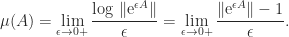
The logarithmic norm of a matrix $A\in\mathbb{C}^{n\times n}$ (also called the logarithmic derivative) is defined by

$\notag \mu(A) = \displaystyle\lim_{\epsilon \to 0+} \frac{ \|I + \epsilon A\| - 1}{\epsilon},$

where the norm is assumed to satisfy $\|I\| = 1$ .

Note that the limit is taken from above. If we take the limit from below then we obtain a generally different quantity: writing $\delta = -\epsilon$ ,

$\notag \displaystyle\lim_{\epsilon \to 0-} \frac{ \|I + \epsilon A\| - 1}{\epsilon} = \lim_{\delta \to 0+} \frac{ \|I - \delta A\| - 1}{-\delta} = -\mu(-A).$

The logarithmic norm is not a matrix norm; indeed it can be negative: $\mu(-I) = -1$ .

The logarithmic norm can also be expressed in terms of the matrix exponential.

Lemma 1. For $A\in\mathbb{C}^{n\times n}$ ,

$\notag \mu(A) = \displaystyle\lim_{\epsilon\to 0+} \frac{\log\, \| \mathrm{e}^{\epsilon A}\|} {\epsilon} = \lim_{\epsilon\to 0+} \frac{\| \mathrm{e}^{\epsilon A}\| - 1} {\epsilon}.$

Properties

We give some basic properties of the logarithmic norm.

It is easy to see that

$\notag -\|A\| \le \mu(A) \le \|A\|. \qquad (1)$

For $z\in\mathbb{C}$ , we define $\mathrm{sign}(z) = z/|z|$ for $z\ne 0$ and $\mathrm{sign}(0) = 0$ .

Lemma 2. For $A,B\in\mathbb{C}^{n\times n}$ and $\lambda\in\mathbb{C}$ ,

$\mu(\lambda A) = |\lambda| \mu\bigl(\mathrm{sign}(\lambda)A\bigr)$ ,

$\mu(A + \lambda I) = \mu(A) + \mathrm{Re}\,\lambda$ ,

$\mu(A + B ) \le \mu(A) + \mu(B)$ ,

$|\mu(A) - \mu(B)| \le \|A - B\|$ .

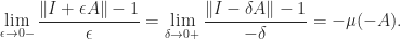
The next result shows the crucial property that $\mu(A)$ features in an easily evaluated bound for the norm of $\mathrm{e}^{At}$ and that, moreover, $\mu(A)$ is the smallest constant that can appear in this bound.

Theorem 3. For $A\in\mathbb{C}^{n\times n}$ and a consistent matrix norm,

$\notag \|\mathrm{e}^{At}\| \le \mathrm{e}^{\mu(A)t}, \quad t\ge0. \qquad (2)$

Moreover,

$\notag \mu(A) = \min\{\, \theta\in\mathbb{R}: \|\mathrm{e}^{At}\| \le \mathrm{e}^{\theta t} ~\mathrm{for~all}~t\ge 0 \,\}.$

Proof. Given any $\delta > 0$ , by Lemma 1 there exists $h > 0$ such that

$\notag \displaystyle\frac{ \| \mathrm{e}^{At}\| - 1}{t} - \mu(A) < \delta, \quad t\in[0,h],$

or

$\notag \| \mathrm{e}^{At}\| \le 1 + (\mu(A) + \delta)t \le \mathrm{e}^{(\mu(A) + \delta)t}, \quad t\in[0,h]$

(since $\mathrm{e}^x \ge 1+x$ for all $x$ ). Then for any integer $k$ , $\|\mathrm{e}^{Atk}\| = \|( \mathrm{e}^{At})^k\| \le \| \mathrm{e}^{At}\|^k \le \mathrm{e}^{(\mu(A) + \delta)tk}$ , and hence $\|\mathrm{e}^{At}\| \le \mathrm{e}^{(\mu(A) + \delta)t}$ holds for all $t\in[0,\infty)$ . Since $\delta$ is arbitrary, it follows that $\|\mathrm{e}^{At}\| \le \mathrm{e}^{\mu(A)t}$ .

Finally, if $\| \mathrm{e}^{At}\| \le \mathrm{e}^{\theta t}$ for all $t\ge 0$ then $(\| \mathrm{e}^{At}\| -1)/t\le (\mathrm{e}^{\theta t}-1)/t$ for all $t\ge0$ and taking $\lim_{t\to 0+}$ we conclude that $\mu(A) \le (d/dt) \mathrm{e}^{\theta t}\mid_{t = 0} \,= \theta$ .

The logarithmic norm was introduced by Dahlquist (1958) and Lozinskii (1958) in order to obtain error bounds for numerical methods for solving differential equations. The bound (2) can alternatively be proved by using differential inequalities (see Söderlind (2006)). Not only is (2) sharper than $\|\mathrm{e}^{At}\| \le \mathrm{e}^{\|A\|t}$ , but $\mathrm{e}^{\|A\|t}$ is increasing in $t$ while $\mathrm{e}^{\mu(A)t}$ potentially decays, since $\mu(A) < 0$ is possible.

The spectral abscissa is defined by

$\notag \alpha(A) = \max \{\, \mathrm{Re} \lambda : \lambda \in \Lambda(A)\,\},$

where $\Lambda(A)$ denotes the spectrum of $A$ (the set of eigenvalues). Whereas the norm bounds the spectral radius ( $\rho(A) \le \|A\|$ ), the logarithmic norm bounds the spectral abscissa, as shown by the next result.

Theorem 4. For $A\in\mathbb{C}^{n\times n}$ and a consistent matrix norm,

$\notag -\mu(-A) \le \alpha(A) \le \mu(A).$

Combining (1) with (2) gives

$\notag -\|A\| \le -\mu(-A) \le \alpha(A) \le \mu(A) \le \|A\|.$

In view of Lemma 1, the logarithmic norm $\mu(A)$ can be expressed as the one-sided derivative of $\|\mathrm{e}^{tA}\|$ at $t = 0$ , so $\mu(A)$ determines the initial rate of change of $\|\mathrm{e}^{tA}\|$ (as well as providing the bound $\mathrm{e}^{\mu(A)t}$ for all $t$ ). The long-term behavior is determined by the spectral abscissa $\alpha(A)$ , since $\|\mathrm{e}^{tA}\| \to 0$ as $t\to\infty$ if and only if $\alpha(A) < 0$ , which can be proved using the Jordan canonical form.

The next result provides a bound on the norm of the inverse of a matrix in terms of the logarithmic norm.

Theorem 5. For a nonsingular matrix $A\in\mathbb{C}^{n\times n}$ and a subordinate matrix norm, if $\mu(A) < 0$ or $\mu(-A) < 0$ then

$\notag \|A^{-1}\| \le \displaystyle\frac{1}{\max\bigl(-\mu(A),-\mu(-A)\bigr)}. \qquad (3)$

Formulas for Logarithmic Norms

Explicit formulas are available for the logarithmic norm s corresponding to the $1$ , $2$ , and $\infty$ -norms.

Theorem 6. For $A\in\mathbb{C}^{n\times n}$ ,

$\notag \begin{aligned} \mu_1(A) &= \max_j \biggl( \sum_{i\ne j} |a_{ij}| + \mathrm{Re}\, a_{jj} \biggr ),\\ \mu_{\infty}(A) &= \max_i \biggl( \sum_{j\ne i} |a_{ij}| + \mathrm{Re}\, a_{ii} \biggr ),\\ \mu_2(A) &= \lambda_{\max}\Bigl( \frac{A+A^*}{2} \Bigr), \qquad (4) \end{aligned}$

where $\lambda_{\max}$ denotes the largest eigenvalue of a Hermitian matrix.

Proof. We have

$\notag \begin{aligned} \mu_{\infty}(A) &= \lim_{\epsilon \to 0+} \frac{ \|I + \epsilon A\|_{\infty} - 1}{\epsilon}\\ &= \lim_{\epsilon \to 0+} \frac{ \max_i \bigl(\sum_{j\ne i} |\epsilon a_{ij}| + |1 + \epsilon a_{ii}| \bigr) -1}{\epsilon}\\ &= \lim_{\epsilon \to 0+} \frac{ \max_i \bigl(\sum_{j\ne i} |\epsilon a_{ij}| + \sqrt{(1 + \epsilon\mathrm{Re}\, a_{ii})^2 + (\epsilon\mathrm{Im}\,a_{ii})^2}\, \bigr) -1}{\epsilon}\\ &= \lim_{\epsilon \to 0+} \frac{ \max_i \bigl( \sum_{j\ne i} |\epsilon a_{ij}| + \epsilon\mathrm{Re}\, a_{ii} + O(\epsilon^2) \bigr)}{\epsilon}\\ &= \max_i \biggl( \sum_{j\ne i} |a_{ij}| + \mathrm{Re}\, a_{ii} \biggr ). \end{aligned}$

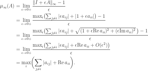
The formula for $\mu_1(A)$ follows, since $\|A\|_1 = \|A^*\|_\infty$ implies $\mu_1(A) = \mu_{\infty}(A^*)$ . For the $2$ -norm, using $\|A\|_2 = \rho(A^*A)^{1/2}$ , we have

$\notag \begin{aligned} \mu_2(A) &= \lim_{\epsilon \to 0+} \frac{ \|I + \epsilon A\|_2 - 1}{\epsilon}\\ &= \lim_{\epsilon \to 0+} \frac{ \rho\bigl( I + \epsilon(A+A^*) + \epsilon^2 A^*A\bigr)^{1/2} -1} {\epsilon}\\ &= \lim_{\epsilon \to 0+} \frac{ 1 + \frac{1}{2}\epsilon\lambda_{\max}(A+A^*) + O(\epsilon^2) -1} {\epsilon}\\ &= \lambda_{\max}\Bigl( \frac{A+A^*}{2} \Bigr). \end{aligned}$

As a special case of (4), if $A$ is normal, so that $A = QDQ^*$ with $Q$ unitary and $D = \mathrm{diag}(\lambda_i)$ , then $\mu_2(A) = \max_i (\lambda_i + \overline{\lambda_i})/2 = \max_i \mathrm{Re} \lambda_i = \alpha(A)$ .

We can make some observations about $\mu_\infty(A)$ for $A\in\mathbb{R}^{n\times n}$ .

If $A\ge 0$ then $\mu_\infty(A) = \|A\|_\infty$ .
$\mu_\infty(A) < 0$ if and only if $a_{ii} < 0$ for all $i$ and $A$ is strictly row diagonally dominant.
For the $\infty$ -norm the bound (3) is the same as a bound based on diagonal dominance except that it is applicable only when the diagonal is one-signed.

For a numerical example, consider the $n\times n$ tridiagonal matrix anymatrix('gallery/lesp'), which has the form illustrated for $n = 6$ by

$\notag A_6 = \left[\begin{array}{cccccc} -5 & 2 & 0 & 0 & 0 & 0\\ \frac{1}{2} & -7 & 3 & 0 & 0 & 0\\ 0 & \frac{1}{3} & -9 & 4 & 0 & 0\\ 0 & 0 & \frac{1}{4} & -11 & 5 & 0\\ 0 & 0 & 0 & \frac{1}{5} & -13 & 6\\ 0 & 0 & 0 & 0 & \frac{1}{6} & -15 \end{array}\right].$

We find that $\alpha(A_6) = -4.55$ and $\mu_2(A_6) = -4.24$ , and it is easy to see that $\mu_1(A_n) = -4.5$ and $\mu_{\infty}(A_n) = -3$ for all $n$ . Therefore Theorem 4 shows that $\mathrm{e}^{At}\to 0$ as $t\to \infty$ and $\mu_1$ gives a faster decaying bound than $\mu_2$ and $\mu_\infty$ .

Now consider the subordinate matrix norm $\|\cdot\|_G$ based on the vector norm $\|x\|_G = (x^*Gx)^{1/2}$ , where $G$ is a Hermitian positive definite matrix. The corresponding logarithmic norm $\mu_G$ can be expressed as the largest eigenvalue of a Hermitian definite generalized eigenvalue problem.

Theorem 7. For $A\in\mathbb{C}^{n\times n}$ ,

$\notag \mu_G(A) = \max\{\, \lambda: \det(GA + A^*G - 2\lambda G) = 0 \,\}.$

Theorem 7 allows us to make a connection with the theory of ordinary differential equations (ODEs)

$\notag y' = f(t,y), \quad f: \mathbb{R} \times \mathbb{R}^n\to \mathbb{R}^n. \qquad (5)$

Let $G\in\mathbb{R}^{n\times n}$ be symmetric positive definite and consider the inner product $\langle x, y \rangle = x^*Gy$ and the corresponding norm defined by 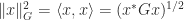$\|x\|_G^2 = \langle x, x \rangle = (x^*Gx)^{1/2}$ . It can be shown that for $A\in\mathbb{R}^{n\times }$ ,

$\notag \mu_G(A) = \max_x \displaystyle\frac{\langle Ax, x\rangle}{\|x\|_G^2}. \qquad (6)$

The function $f$ satisfies a one-sided Lipschitz condition if there is a function $v(t)$ such that

$\langle f(t,y) - f(t,z), y - z \rangle \le v(t) \|y-z\|^2$

for all $y,z$ in some region and all $a\le t \le b$ . For the linear differential equation with $f(t,y) = A(t)y$ in (5), using (6) we obtain

$\langle f(t,y) - f(t,z), y - z \rangle = \langle A(t)(y-z), y - z \rangle \le \mu_G(A(t)) \|y-z\|_G^2,$

and so the logarithmic norm $\mu_G(A(t))$ can be taken as a one-sided Lipschitz constant. This observation leads to results on contractivity of ODEs; see Lambert (1991) for details.

Notes

For more on the use of the logarithmic norm in differential equations see Coppel (1965) and Söderlind (2006).

The proof of Theorem 3 is from Hinrichsen and Pritchard (2005).

References

This is a minimal set of references, which contain further useful references within.

W. A. Coppel, Stability and Asymptotic Behavior of Differential Equations}. D. C. Heath and Company, Boston, MA. USA, 1965.
Germund Dahlquist. Stability and Error Bounds in the Numerical Integration of Ordinary Differential Equations. PhD thesis, Royal Inst. of Technology, Stockholm, Sweden, 1958.
Diederich Hinrichsen and Anthony J. Pritchard. Mathematical Systems Theory I. Modelling, State Space Analysis, Stability and Robustness. Springer-Verlag, Berlin, Germany, 2005.
J. D. Lambert. Numerical Methods for Ordinary Differential Systems. The Initial Value Problem. John Wiley, Chichester, 1991.
Gustaf Söderlind, The Logarithmic Norm. History and Modern Theory. BIT, 46(3):631–652, 2006.
Torsten Ström. On Logarithmic Norms. SIAM J. Numer. Anal., 12(5):741–753, 1975.

What Is a Tridiagonal Matrix?

A tridiagonal matrix is a square matrix whose elements are zero away from the main diagonal, the subdiagonal, and the superdiagonal. In other words, it is a banded matrix with upper and lower bandwidths both equal to $1$ . It has the form

$\notag A = \begin{bmatrix} d_1 & e_1 & & &\\ c_2 & d_2 & e_2 & &\\ & c_3 & \ddots & \ddots &\\ & & \ddots & \ddots & e_{n-1}\\ & & & c_n & d_n \end{bmatrix} \in\mathbb{C}^{n\times n}.$

An important example is the matrix $T_n$ that arises in discretizating the Poisson partial differential equation by a standard five-point operator, illustrated for $n = 5$ by

$\notag T_5 = \left[ \begin{array}{@{}*{4}{r@{\mskip10mu}}r} 4 & -1 & & & \\ -1 & 4 & -1 & & \\ & -1 & 4 & -1 & \\ & & -1 & 4 & -1 \\ & & & -1 & 4 \end{array}\right].$

It is symmetric positive definite, diagonally dominant, a Toeplitz matrix, and an $M$ -matrix.

Tridiagonal matrices have many special properties and various algorithms exist that exploit their structure.

Symmetrization

It can be useful to symmetrize a matrix by transforming it with a diagonal matrix. The next result shows when symmetrization is possible by similarity.

Theorem 1. If $A\in\mathbb{R}^{n\times n}$ is tridiagonal and $c_i e_{i-1} > 0$ for all $i$ then there exists a diagonal $D\in\mathbb{R}^{n\times n}$ with positive diagonal elements such that $D^{-1}AD$ is symmetric, with $(i-1,i)$ element $(c_ie_{i-1})^{1/2}$ .

Proof. Let $D = \mathrm{diag}(\omega_i)$ . Equating $(i,i-1)$ and $(i-1,i)$ elements in the matrix $D^{-1}AD$ gives

$\notag c_i \displaystyle\frac{\omega_{i-1}}{\omega_i} = e_{i-1} \displaystyle\frac{\omega_i}{\omega_{i-1}}, \quad i = 2:n, \qquad(1)$

or

$\notag \biggl(\displaystyle\frac{\omega_{i-1}}{\omega_i}\biggr)^2 = \frac{e_{i-1} }{c_i}, \quad i = 2:n. \qquad (2)$

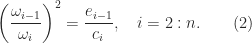
As long as $c_i e_{i-1} > 0$ for all $i$ we can set $\omega_1 = 1$ and solve (2) to obtain real, positive $\omega_i$ , $i = 2:n$ . The formula for the off-diagonal elements of the symmetrized matrix follows from (1) and (2).

LU Factorization

The LU factors of a tridiagonal matrix are bidiagonal:

$\notag L = \begin{bmatrix} 1 & & & & \\ \ell_2 & 1 & & & \\ & \ell_3 & 1 & & \\ & & \ddots & \ddots & \\ & & & \ell_n & 1 \end{bmatrix}, \quad U = \begin{bmatrix} u_1 & e_1 & & & \\ & u_2 & e_2 & & \\ & & \ddots & \ddots & \\ & & & \ddots & e_{n-1}\\ & & & & u_n \end{bmatrix}. \qquad (3)$

The equation $A = LU$ gives the recurrence

$\notag u_1 = d_1, \qquad \ell_i = c_i/u_{i-1}, \quad u_i = d_i - \ell_i e_{i-1}, \quad i=2\colon n. \qquad (4)$

The recurrence breaks down with division by zero if one of the leading principal submatrices $A(1:k,1:k)$ , $k = 1:n-1$ , is singular. In general, partial pivoting must be used to ensure existence and numerical stability, giving a factorization $PA = LU$ where $L$ has at most two nonzeros per column and $U$ has an extra superdiagonal. The growth factor $\rho_n$ is easily seen to be bounded by $2$ .

For a tridiagonal Toeplitz matrix

$\notag T_n(c,d,e) = \begin{bmatrix} d & e & & \\ c & d & \ddots & \\ & \ddots & \ddots & e \\ & & c & d \end{bmatrix} \in\mathbb{C}^{n\times n} \qquad (5)$

the elements of the LU factors converge as $n\to\infty$ if $A$ is diagonally dominant.

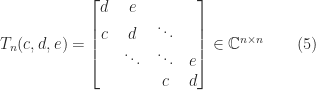
Theorem 2. Suppose that $T_n(c,d,e)$ has an LU factorization with LU factors (3) and that $ce > 0$ and $|d| \ge 2\sqrt{ce}$ . Then $|u_j|$ decreases monotonically and

$\notag \lim_{n\to \infty}u_n = \frac{1}{2} \Bigl(d + \mathrm{sign}(d) \sqrt{ d^2 - 4ce } \Bigr).$

From (4), it follows that under the conditions of Theorem 2, $|\ell_i|$ increases monotonically and $\lim_{n\to\infty}\ell_n = e/\lim_{n\to\infty}u_n$ . Note that the conditions of Theorem 2 are satisfied if $A$ is diagonally dominant by rows, since $ce> 0$ implies $d \ge c + e \ge 2\sqrt{ce}$ . Note also that if we symmetrize $A$ using Theorem 1 then we obtain the matrix $T_n(\sqrt{ce},d, \sqrt{ce})$ , which is irreducibly diagonally dominant and hence positive definite if $d > 0$ .

Inverse

The inverse of a tridiagonal matrix is full, in general. For example,

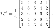
$\notag T_5(-1,3,-1)^{-1} = \left[\begin{array}{rrrrr} 3 & -1 & 0 & 0 & 0\\ -1 & 3 & -1 & 0 & 0\\ 0 & -1 & 3 & -1 & 0\\ 0 & 0 & -1 & 3 & -1\\ 0 & 0 & 0 & -1 & 3 \end{array}\right]^{-1} = \frac{1}{144} \left[\begin{array}{ccccc} 55 & 21 & 8 & 3 & 1 \\ 21 & 63 & 24 & 9 & 3 \\ 8 & 24 & 64 & 24 & 8 \\ 3 & 9 & 24 & 63 & 21\\ 1 & 3 & 8 & 21 & 55 \end{array}\right].$

Since an $n\times n$ tridiagonal matrix depends on only $3n-2$ parameters, the same must be true of its inverse, meaning that there must be relations between the elements of the inverse. Indeed, in $T_5(-1,3,-1)^{-1}$ any $2\times 2$ submatrix whose elements lie in the upper triangle is singular, and the $(1:3,3:5)$ submatrix is also singular. The next result explains this special structure. We note that a tridiagonal matrix is irreducible if $a_{i+1,i}$ and $a_{i,i+1}$ are nonzero for all $i$ .

Theorem 3. If $A\in\mathbb{C}^{n\times n}$ is tridiagonal, nonsingular, and irreducible then there are vectors $u$ , $v$ , $x$ , and $y$ , all of whose elements are nonzero, such that

$\notag (A^{-1})_{ij} = \begin{cases} u_iv_j, & i\le j,\\ x_iy_j, & i\ge j.\\[4pt] \end{cases}$

The theorem says that the upper triangle of the inverse agrees with the upper triangle of a rank- $1$ matrix ( $uv^T$ ) and the lower triangle of the inverse agrees with the lower triangle of another rank- $1$ matrix ( $xy^T$ ). This explains the singular submatrices that we see in the example above.

If a tridiagonal matrix $A$ is reducible with $a_{k,k+1} = 0$ then it has the block form

$\notag \begin{bmatrix} A_{11} & 0 \\ A_{21} & A_{22} \end{bmatrix},$

where $A_{21} = a_{k+1,k}e_1e_k^T$ , and so

$\notag \begin{bmatrix} A_{11}^{-1} & 0 \\ - A_{22}^{-1} A_{21} A_{11}^{-1} & A_{22}^{-1} \end{bmatrix},$

in which the $(2,1)$ block is rank $1$ if $a_{k+1,k}\ne 0$ . This blocking can be applied recursively until Theorem 1 can be applied to all the diagonal blocks.

The inverse of the Toeplitz tridiagonal matrix $T_n(a,b,c)$ is known explicitly; see Dow (2003, Sec. 3.1).

Eigenvalues

The most widely used methods for finding eigenvalues and eigenvectors of Hermitian matrices reduce the matrix to tridiagonal form by a finite sequence of unitary similarity transformations and then solve the tridiagonal eigenvalue problem. Tridiagonal eigenvalue problems also arise directly, for example in connection with orthogonal polynomials and special functions.

The eigenvalues of the Toeplitz tridiagonal matrix $T_n(c,d,e)$ in (5) are given by

$\notag d + 2 (ce)^{1/2} \cos\biggl( \displaystyle\frac{k \pi}{n+1} \biggr), \quad k = 1:n. \qquad (6)$

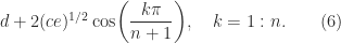
The eigenvalues are also known for certain variations of the symmetric matrix $T_n(c,d,c)$ in which the $(1,1)$ and $(n,n)$ elements are modified (Gregory and Karney, 1969).

Some special results hold for the eigenvalues of general tridiagonal matrices. A matrix is derogatory if an eigenvalue appears in more than one Jordan block in the Jordan canonical form, and nonderogatory otherwise.

Theorem 4. If $A\in\mathbb{C}^{n\times n}$ is an irreducible tridiagonal matrix then it is nonderogatory.

Proof. Let $G = A - \lambda I$ , for any $\lambda$ . The matrix $G(1:n-1,2:n)$ is lower triangular with nonzero diagonal elements $e_1, \dots, e_{n-1}$ and hence it is nonsingular. Therefore $G$ has rank at least $n-1$ for all $\lambda$ . If $A$ were derogatory then the rank of $G$ would be at most $n-2$ when $\lambda$ is an eigenvalue, so $A$ must be nonderogatory.

Corollary 5. If $A\in\mathbb{R}^{n\times n}$ is tridiagonal with $c_i e_{i-1} > 0$ for all $i$ then the eigenvalues of $A$ are real and simple.

Proof. By Theorem 1 the eigenvalues of $A$ are those of the symmetric matrix $S = D^{-1}AD$ and so are real. The matrix $S$ is tridiagonal and irreducible so it is nonderogatory by Theorem 4, which means that its eigenvalues are simple because it is symmetric.

The formula (6) confirms the conclusion of Corollary 5 for tridiagonal Toeplitz matrices.

Corollary 5 guarantees that the eigenvalues are distinct but not that they are well separated. The spacing of the eigenvalues in (6) clearly reduces as $n$ increases. Wilkinson constructed a symmetric tridiagonal matrix called $W_n^+$ , defined by

$\notag \begin{aligned} d_i &= \frac{n+1}{2} - i = d_{n-i+1}, \quad i = 1:n/2, \qquad d_{(n+1)/2} = 0 \quad \mathrm{if}~n~\mathrm{is~odd}, \\ c_i &= e_{i-1} = 1. \end{aligned}$

For example,

$\notag W_5^+ = \left[\begin{array}{ccccc} 2 & 1 & 0 & 0 & 0\\ 1 & 1 & 1 & 0 & 0\\ 0 & 1 & 0 & 1 & 0\\ 0 & 0 & 1 & 1 & 1\\ 0 & 0 & 0 & 1 & 2 \end{array}\right].$

Here are the two largest eigenvalues of $W_{21}^+$ , as computed by MATLAB.

>> A = anymatrix('matlab/wilkinson',21); 
>> e = eig(A); e([20 21])
ans =
  10.746194182903322
  10.746194182903393

These eigenvalues (which are correct to the digits shown) agree almost to the machine precision.

Notes

Theorem 2 is obtained for symmetric matrices by Malcolm and Palmer (1974), who suggest saving work in computing the LU factorization by setting $u_j = u_k$ for $j > k$ once $u_k$ is close enough to the limit.

A sample reference for Theorem 3 is Ikebe (1979), which is one of many papers on inverses of banded matrices.

The eigenvectors of a symmetric tridiagonal matrix satisfy some intricate relations; see Parlett (1998, sec. 7.9).

References

This is a minimal set of references, which contain further useful references within.

Murray Dow, Explicit Inverses of Toeplitz and Associated Matrices, ANZIAM J. 44, E185–E215, 2003.
Robert Gregory and David Karney, A Collection of Matrices for Testing Computational Algorithms, Wiley, 1969.
Yasuhiko Ikebe, On inverses of Hessenberg matrices. Linear Algebra Appl., 24:93–97, 1979.
Michael A. Malcolm and John Palmer, A Fast Method for Solving a Class of Tridiagonal Linear Systems, Comm. ACM 17, 14–17, 1974.
Beresford Parlett, The Symmetric Eigenvalue Problem, Society for Industrial and Applied Mathematics, Philadelphia, PA, USA, 1998.
J. H. Wilkinson, The Algebraic Eigenvalue Problem, Oxford University Press, 1965, Section 5.45.

Month: January 2022

What Is the Second Difference Matrix?

Cholesky Factorization

Determinant, Inverse, Condition Number

Eigenvalues and Eigenvectors

Variations

Notes

References

Related Blog Posts

What Is the Frank Matrix?

Determinant

Inverse and Condition Number

Eigenvalues

Notes

References

Related Blog Posts

What Is the Logarithmic Norm?

Properties

Formulas for Logarithmic Norms

Notes

References

Related Blog Posts

What Is a Tridiagonal Matrix?

Symmetrization

LU Factorization

Inverse

Eigenvalues

Notes

References

Related Blog Posts

Cholesky Factorization

Determinant, Inverse, Condition Number

Eigenvalues and Eigenvectors

Variations

Notes

References

Related Blog Posts

Share this:

Determinant

Inverse and Condition Number

Eigenvalues

Notes

References

Related Blog Posts

Share this:

Properties

Formulas for Logarithmic Norms

Notes

References

Related Blog Posts

Share this:

Symmetrization

LU Factorization

Inverse

Eigenvalues

Notes

References

Related Blog Posts

Share this: