A matrix is a rectangular array of numbers on which certain algebraic operations are defined. Matrices provide a convenient way of encapsulating many numbers in a single object and manipulating those numbers in useful ways.
An 


An example of a square matrix is
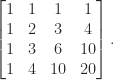
This matrix is symmetric: 


Addition of matrices of the same dimensions is defined in the obvious way: by adding the corresponding entries.
Multiplication of matrices requires the inner dimensions to match. The product of an 


When 


The inverse of a square matrix 


The transpose of an 


In linear algebra, a matrix represents a linear transformation between two vector spaces in terms of particular bases for each space.
Vectors and scalars are special cases of matrices: column vectors are 


Many programming languages and problem solving environments support arrays. It is important to note that operations on arrays are typically defined componentwise, so that, for example, multiplying two arrays multiplies the corresponding pairs of entries, which is not the same as matrix multiplication. The quintessential programming environment for matrices is MATLAB, in which a matrix is the core data type.
It is possible to give meaning to a matrix with one or both dimensions zero. MATLAB supports such empty matrices. Matrix multiplication generalizes in a natural way to allow empty dimensions:
>> A = zeros(0,2)*zeros(2,3)
A =
0x3 empty double matrix

>> A = zeros(2,0)*zeros(0,3)
A =
0     0     0
0     0     0
In linear algebra and numerical analysis, matrices are usually written with a capital letter and vectors with a lower case letter. In some contexts matrices are distinguished by boldface.
The term matrix was coined by James Joseph Sylvester in 1850. Arthur Cayley was the first to define matrix algebra, in 1858.
References
- Arthur Cayley, A Memoir on the Theory of Matrices, Philos. Trans. Roy. Soc. London 148, 17–37, 1858.
- Nicholas J. Higham, Sylvester’s Influence on Applied Mathematics, Mathematics Today 50, 202–206, 2014. A version of the article with an extended bibliography containing additional historical references is available as a MIMS EPrint.
- Roger A. Horn and Charles R. Johnson, Matrix Analysis, second edition, Cambridge University Press, 2013. My review of the second edition.
Related Blog Posts
- Empty Matrices in MATLAB (2016).
This article is part of the “What Is” series, available from https://nhigham.com/category/what-is and in PDF form from the GitHub repository https://github.com/higham/what-is.

 and for arbitrary precision evaluation of the exponential and logarithm.
 from
from  to
to  to
to  , the backward error in
  such that
  , for some appropriate measure of size. There can be many

 of two vectors the backward error of an approximation
  can be defined as
 . It can be shown that
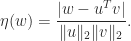
 is clearly unsymmetric in that
  is perturbed but
  is not. If
  and
and  and no explicit formula is available for
  of two
  is unlikely to be of rank 1, so
  is not in general possible for any
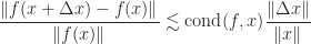
  is bounded in terms of the backward error
  by
by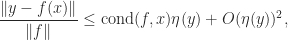

 . More correctly, this is the condition number with respect to inversion, because a relative change to
  can change
  by a relative amount as much as, but no more than, about
  for small
  is also the condition number for a linear system
  (exactly if
  are the data).
 for any norm for which
  (most common norms, but not the Frobenius norm, have this property) and that
 , with approximate equality for some
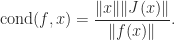
  can be given in terms of the Jacobian matrix,
 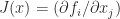 :
:
 , so
, so  . Hence, for example,
  .
. is a simple (non-repeated) root of the polynomial
  then the data is the vector of coefficients
 ![a = [a_n,\dots,a_0]^T](https://s0.wp.com/latex.php?latex=a+%3D+%5Ba_n%2C%5Cdots%2Ca_0%5D%5ET&bg=ffffff&fg=222222&s=0&c=20201002) . It can be shown that the condition number of the root
. It can be shown that the condition number of the root  -norm,

 produce small changes in
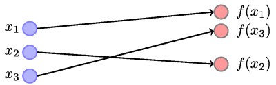
 and
and  illustrates).
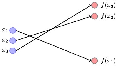
 .
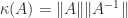
. condition number
 ) of the posts available on GitHub in the repository