Numerical stability concerns how errors introduced during the execution of an algorithm affect the result. It is a property of an algorithm rather than the problem being solved. I will assume that the errors under consideration are rounding errors, but in principle the errors can be from any source.
Consider a scalar function 


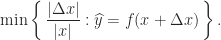
If 


An algorithm that always produces a small backward error is called backward stable. In a backward stable algorithm the errors introduced during the algorithm have the same effect as a small perturbation in the data. If the backward error is the same size as any uncertainty in the data then the algorithm produces as good a result as we can expect.
If 
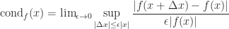
is the condition number of 
The definition of 
If

with 

With these definitions in hand, we can turn to the meaning of the term numerically stable. Depending on the context, numerical stability can mean that an algorithm is (a) backward stable, (b) forward stable, or (c) mixed backward–forward stable.
For some problems, backward stability is difficult or impossible to achieve, so numerical stability has meaning (b) or (c). For example, let 


We briefly mention some other relevant points.
- What is the data? For a linear system
the data is
or
, or both. For a nonlinear function we need to consider whether problem parameters are data; for example, for
are the
and the
constants or are they data, like
- We have measured perturbations in a relative sense. Absolute errors can also be used.
- For problems whose inputs are matrices or vectors we need to use norms or componentwise measures.
- Some algorithms are only unconditionally numerically stable, that is, they are numerically stable for some subset of problems. For example, the normal equations method for solving a linear least squares problem is forward stable for problems with a large residual.
References
This is a minimal set of references, which contain further useful references within.
- Robert M. Corless and Nicolas Fillion, A Graduate Introduction to Numerical Methods from the Viewpoint of Backward Error Analysis, Springer, New York, 2013. My review of this book.
- Nicholas J. Higham, Accuracy and Stability of Numerical Algorithms, second edition, Society for Industrial and Applied Mathematics, Philadelphia, PA, USA, 2002.
Related Blog Posts
- What Is a Condition Number? (2020)
- What Is Backward Error? (2020)
This article is part of the “What Is” series, available from https://nhigham.com/category/what-is and in PDF form from the GitHub repository https://github.com/higham/what-is.
