How and How Not to Compute a Relative Error

The relative error in a scalar $y$ as an approximation to a scalar $x$ is the absolute value of $e = (x-y)/x$ . I recently came across a program in which $e$ had been computed as $1 - y/x$ . It had never occurred to me to compute it this way. The second version is slightly easier to type, requiring no parentheses, and it has the same cost of evaluation: one division and one subtraction. Is there any reason not to use this parenthesis-free expression?

Consider the accuracy of the evaluation, using the standard model of floating point arithmetic, which says that $fl(x \mathbin{\mathrm{op}} y) = (x \mathbin{\mathrm{op}} y)(1+\delta)$ with $|\delta| \le u$ , where $\mathrm{op}$ is any one of the four elementary arithmetic operations and $u$ is the unit roundoff. For the expression $e_1 = (x-y)/x$ we obtain, with a hat denoting a computed quantity,

$\widehat{e_1} = \displaystyle\left(\frac{x-y}{x}\right) (1+\delta_1)(1+\delta_2), \qquad |\delta_i| \le u, \quad i = 1, 2.$

It follows that

$\left| \displaystyle\frac{e - \widehat{e_1}}{e} \right| \le 2u + u^2.$

Hence $e_1$ is computed very accurately.

For the alternative expression, $e_2 = 1 - y/x$ , we have

$\widehat{e_2} = \left(1 - \displaystyle\frac{y}{x}(1+\delta_1)\right) (1+\delta_2), \qquad |\delta_i| \le u, \quad i = 1, 2.$

After a little manipulation we obtain the bound

$\left| \displaystyle\frac{e - \widehat{e_2}}{e} \right| \le u + \left|\displaystyle\frac{1-e}{e}\right|(u + u^2).$

The bound on the relative error in $\widehat{e_2}$ is of order $|(1-e)/e|u$ , and hence is very large when $|e| \ll 1$ .

To check these bounds we carried out a MATLAB experiment. For 500 single precision floating point numbers $y$ centered on $x = 3$ , we evaluated the relative error of $y$ as an approximation to $x$ using the two formulas. The results are shown in this figure, where an ideal error is of order $u \approx 6\times 10^{-8}$ . (The MATLAB script that generates the figure is available as this gist.)

As expected from the error bounds, the formula $1-y/x$ is very inaccurate when $y$ is close to $x$ , whereas $(x-y)/x$ retains its accuracy as $y$ approaches $x$ .

Does this inaccuracy matter? Usually, we are concerned only with the order of magnitude of an error and do not require an approximation with many correct significant figures. However, as the figure shows, for the formula $|1-y/x|$ even the order of magnitude is incorrect for $y$ very close to $x$ . The standard formula $|x-y|/|x|$ should be preferred.

The Rise of Mixed Precision Arithmetic

For the last 30 years, most floating point calculations in scientific computing have been carried out in 64-bit IEEE double precision arithmetic, which provides the elementary operations of addition, subtraction, multiplication, and division at a relative accuracy of about $10^{-16}$ . We are now seeing growing use of mixed precision, in which different floating point precisions are combined in order to deliver a result of the required accuracy at minimal cost.

Single precision arithmetic (32 bits) is an attractive alternative to double precision because it halves the costs of storing and transferring data, and on Intel chips the SSE extensions allow single precision arithmetic to run twice as fast as double.

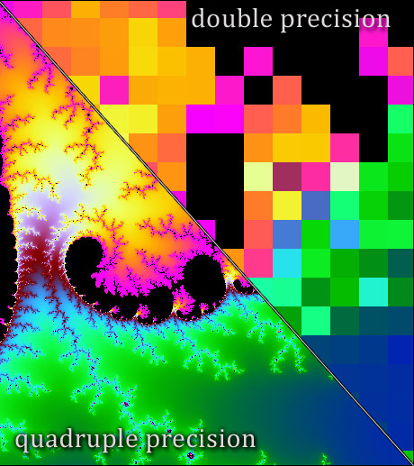
” /> The Mandelbrot set computed in double and quadruple precision. Image taken from https://www.thasler.com/blog/blog/glsl-part5.

Quadruple precision arithmetic, which was included in the 2008 revision of the IEEE standard, is supported by some compilers, and it can be implemented in terms of double precision arithmetic via double-double arithmetic. Arbitrary precision floating point arithmetic is available through, for example, the GNU MPFR library, the mpmath library for Python, the core data type BigFloat in the new language Julia, VPA arithmetic in the MATLAB Symbolic Math Toolbox, or the Advanpix Multiprecision Computing Toolbox for MATLAB.

Half precision arithmetic, in which a number occupies 16 bits, is supported by the IEEE standard for storage but not for computation. It has been argued that for deep learning half precision, with its relative accuracy of about $10^{-4}$ , is good enough for training and running neural networks. Here are some of the ways in which extra precision is currently being used.

Iterative refinement, in the traditional form that first became popular in the 1960s, improves the quality of an approximate solution to a linear system via updates obtained from residuals computed in extra precision.
When an algorithm suffers instability it may be possible to overcome it by using extra precision in just a few, key places. This has been done recently in eigensolvers and for matrix orthonormalization.
Any iterative algorithm that accepts an arbitrary starting point can be run once at a given precision and the solution used to “warm start” a second run of the same algorithm at higher precision. This idea has been used recently in linear programming.
Numerical integration of differential equations over long time periods may need higher precision in order to allow the phenomena of interest to be observed. A recent example is in the study of Kerr (rotating) black holes, where the underlying hyperbolic partial differential equation is solved using quadruple precision arithmetic running on GPUs.
When one is developing error bounds or testing algorithms, one needs in principle the exact solution. In practice, a solution computed at high precision and rounded to the working precision is usually adequate, and this is an approach I frequently use in my work in numerical linear algebra.

As the relative costs and ease of computing at different precisions evolve, due to changing architectures and software, as well as the disruptive influence of accelerators such as GPUs, we will see an increasing development and use of mixed precision algorithms. In some ways this is analogous to the increasing interoperability of programming languages (illustrated by C++, Julia, and Python, for example): one uses the main tool (precision) one would like to work with and brings in other tools (precisions) as necessary in order to complete the task.

Update: linear programming link updated December 18, 2018.

Tiny Relative Errors

Let $x\ne0$ and $y$ be distinct floating point numbers. How small can the relative difference between $x$ and $y$ be? For IEEE double precision arithmetic the answer is $u = 2^{-53} \approx 1.1 \times 10^{-16}$ , which is called the unit roundoff.

What if we now let $x$ and $y$ be vectors and define the relative difference as $d(x,y) = \|x-y\|_{\infty}/\|x\|_{\infty}$ , where the infinity norm is $\|x\|_{\infty} = \max_i |x_i|$ ? It does not seem to be well known that $d(x,y)$ can be much less than $u$ . I have observed this phenomenon numerous times over the years but had not previously stopped to wonder how it could happen. An example is

$x = \begin{bmatrix}1 \\ 10^{-22} \end{bmatrix}, \quad y = \begin{bmatrix}1 \\ 2\times 10^{-22} \end{bmatrix}, \quad d(x,y) = 10^{-22}$ .

Notice that the largest element(s) in magnitude of $x$ agrees with the corresponding element(s) of $y$ . This is, in fact, the only way that $d(x,y) < u$ is possible.

Theorem (Dingle & Higham, 2013).
Let $x\ne0$ and $y$ be $n$ -vectors of normalized floating point numbers.
If $d(x,y) < u$ then $x_k = y_k$ for all $k$ such that $|x_k| = \|x\|_{\infty}$ .

This result, and the scalar case mentioned above, are proved in

Nicholas J. Higham and Nicholas J. Dingle, Reducing the Influence of Tiny Normwise Relative Errors on Performance Profiles, MIMS EPrint 2011.90; to appear in ACM Trans. Math. Soft.

Performance profiles, introduced by Dolan and Moré in 2002, are a popular way to compare competing algorithms according to particular measures of performance, such as relative error or execution time. We show in the paper above that tiny relative errors can result in misleading performance profiles and show how a simple transformation of the data can lead to much more useful profiles. For more, see the paper or the talk Numerical Issues in Testing Linear Algebra Algorithms that I gave at the SIAM Conference on Computational Science and Engineering in Boston last week.

Share this:

Share this:

Share this: