Matrices arising in applications often have diagonal elements that are large relative to the off-diagonal elements. In the context of a linear system this corresponds to relatively weak interactions between the different unknowns. We might expect a matrix with a large diagonal to be assured of certain properties, such as nonsingularity. However, to ensure nonsingularity it is not enough for each diagonal element to be the largest in its row. For example, the matrix
![\notag \left[\begin{array}{rrr} 3 & -1 & -2\\ -2 & 3 & -1\\ -2 & -1 & 3 \end{array}\right] \qquad (1)](https://s0.wp.com/latex.php?latex=%5Cnotag++%5Cleft%5B%5Cbegin%7Barray%7D%7Brrr%7D+++++3+%26+-1+%26+-2%5C%5C++++-2+%26++3+%26+-1%5C%5C++++-2+%26+-1+%26++3+++%5Cend%7Barray%7D%5Cright%5D+%5Cqquad+%281%29+&bg=ffffff&fg=222222&s=0&c=20201002)
is singular because ![[1~1~1]^T](https://s0.wp.com/latex.php?latex=%5B1%7E1%7E1%5D%5ET&bg=ffffff&fg=222222&s=0&c=20201002)
A matrix 
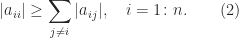
It is strictly diagonally dominant by rows if strict inequality holds in (2) for all 


Diagonal dominance on its own is not enough to ensure nonsingularity, as the matrix (1) shows. Strict diagonal dominance does imply nonsingularity, however.
Theorem 1.
If
Proof. Since
let
and choose
so that
. Then the
which gives
Using (2), we have
Therefore
and so


Diagonal dominance plus two further conditions is enough to ensure nonsingularity. We need the notion of irreducibility. A matrix 

with 

Theorem 2.
If
for some
Proof. The proof is by contradiction. Suppose there exists
such that
. Define
The
Hence for
,
The set
is nonempty, because if it were empty then we would have
for all
and if there is strict inequality in
, then putting
, which is a contradiction. Hence as long as
for some
, we obtain
, which contradicts the diagonal dominance. Therefore we must have
for all
. This means that all the rows indexed by
have zeros in the columns indexed by


The obvious analogue of Theorem 2 holds for column diagonal dominance.
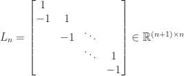
As an example, the 
![\notag T_n = \left[\begin{array}{@{\mskip 5mu}c*{4}{@{\mskip 15mu} r}@{\mskip 5mu}} 2 & -1 & & & \\ -1 & 2 & -1 & & \\ & -1 & 2 & \ddots & \\ & & \ddots & \ddots & -1\\ & & & -1 & 2 \end{array}\right], \qquad (5)](https://s0.wp.com/latex.php?latex=%5Cnotag++T_n+%3D+%5Cleft%5B%5Cbegin%7Barray%7D%7B%40%7B%5Cmskip+5mu%7Dc%2A%7B4%7D%7B%40%7B%5Cmskip+15mu%7D+r%7D%40%7B%5Cmskip+5mu%7D%7D++++++2+%26+++-1++%26++++++++++%26+++++++++%26+%5C%5C+++++-1+%26++++2++%26++-1++++++%26+++++++++%26+%5C%5C++++++++%26++++-1+%26+++2++++++%26++%5Cddots+%26+%5C%5C++++++++%26+++++++%26++%5Cddots++%26++%5Cddots+%26+-1%5C%5C++++++++%26+++++++%26++++++++++%26++-1+++++%26+2++++++++++++%5Cend%7Barray%7D%5Cright%5D%2C+%5Cqquad+%285%29+&bg=ffffff&fg=222222&s=0&c=20201002)
is row diagonally dominant with strict inequality in the first and last diagonal dominance relations. It can also be shown to be irreducible and so it is nonsingular by Theorem 2. If we replace 


then 

Since in general 


Relation to Gershgorin’s Theorem
Theorem 1 can be used to obtain information about the location of the eigenvalues of a matrix. Indeed if 

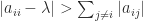
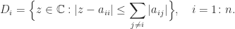
Theorem 3 (Gershgorin’s theorem).
The eigenvalues of
discs in the complex plane
If 

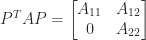
Generalized Diagonal Dominance
In some situations

is not diagonally dominant by rows or columns but

is strictly diagonally dominant by rows.
A matrix 


It is easy to see that if
It can be shown that 

is an 
Block Diagonal Dominance
A matrix 


Analogues of Theorems 1 and 2 giving conditions under which block diagonal dominance implies nonsingularity are given by Feingold and Varga (1962).
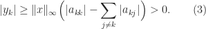
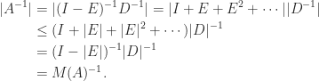
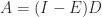
Bounding the Inverse
If a matrix is strictly diagonally dominant then we can bound its inverse in terms of the minimum amount of diagonal dominance. For full generality, we state the bound in terms of generalized diagonal dominance.
Theorem 4.
If
where
.
Proof. Assume first that
. Let
satisfy
and let
. Applying (3) gives
. The result is obtained on applying this bound to
.
.

Another bound for 


This bound implies that 
An upper bound also holds for block diagonal dominance.
Theorem 5.
If
where
.

It is interesting to note that the inverse of a strictly row diagonally dominant matrix enjoys a form of diagonal dominance, namely that the largest element in each column is on the diagonal.
Theorem 6.
If
satisfies
for all
Proof. For
. Let
. Taking absolute values in
gives
or
, since
. This inequality holds for all
, which gives the result.

Historical Remarks
Theorems 1 and 2 have a long history and have been rediscovered many times. Theorem 1 was first stated by Lévy (1881) with additional assumptions. In a short but influential paper, Taussky (1949) pointed out the recurring nature of the theorems and gave simple proofs (our proof of Theorem 2 is Taussky’s). Schneider (1977) attributes the surge in interest in matrix theory in the 1950s and 1960s to Taussky’s paper and a few others by her, Brauer, Ostrowski, and Wielandt. The history of Gershgorin’s theorem (published in 1931) is intertwined with that of Theorems 1 and 2; see Varga’s 2004 book for details.
Theorems 4 and 5 are from Varah (1975) and Theorem 6 is from Ostrowski (1952).
References
This is a minimal set of references, which contain further useful references within.
- David G. Feingold and Richard S. Varga, Block Diagonally Dominant Matrices and Generalizations of the Gerschgorin Circle Theorem, Pacific J. Math. 12(4), 1241–1250, 1962.
- A. M. Ostrowski, Note on Bounds for Determinants with Dominant Principal Diagonal, Proc. Amer. Math. Soc. 3, 260–30, 1952.
- Hans Schneider, Olga Taussky-Todd’s Influence on Matrix Theory and Matrix Theorists: A Discursive Personal Tribute, Linear and Multilinear Algebra 5, 197–224, 1977.
- Olga Taussky, A Recurring Theorem on Determinants, Amer. Math. Monthly 56(2), 672–676, 1949.
- J. M. Varah, A Lower Bound for the Smallest Singular Value of a Matrix, Linear Algebra Appl. 11, 3–5, 1975.
- Richard Varga, Geršgorin and His Circles, Springer-Verlag, Berlin, 2004.
Related Blog Posts
This article is part of the “What Is” series, available from https://nhigham.com/category/what-is and in PDF form from the GitHub repository https://github.com/higham/what-is.

Nick, I guess one needs the strict inequality in Equation (2).
(2) is diagonal dominance. (2) with strict inequality for all i is strict diagonal dominance.
Ok, sorry. I think I went too quickly.
Hello Nick,
Nice post. There is an important class of diagonally dominant (DD) matrices that just miss being M-matrices. I’ll refer to them as Q matrices, the name bestowed upon them by probabilists in their study of continuous-time Markov chains. Like M-matrices, the diagonal elements are positive and the off-diagonal elements are non-positive. But they are singular. Are you aware of a specific name for this class of DD matrices outside of Q matrices?
Hi Rich. What you are describing sounds like minus a transition intensity matrix, which has zero row sums and which comes up as a generator for a Markov chain.