In many situations we need to estimate or bound the norm of the inverse of a matrix, for example to compute an error bound or to check whether an iterative process is guaranteed to converge. This is the same problem as bounding the condition number 

We denote by 

It will be useful to note that
![\notag \left[\begin{array}{crrrr} 1 & -\theta & -\theta & -\theta & -\theta\\ & 1 & -\theta & -\theta & -\theta\\ & & 1 & -\theta & -\theta\\ & & & 1 & -\theta\\ & & & & 1 \end{array}\right]^{-1} = \left[\begin{array}{ccccc} 1 & \theta & \theta(1+\theta) & \theta(1+\theta)^2 & \theta(1+\theta)^3\\ & 1 & \theta & \theta(1+\theta) & \theta(1+\theta)^2\\ & & 1 & \theta & \theta(1+\theta)\\ & & & 1 & \theta\\ & & & & 1 \end{array}\right]](https://s0.wp.com/latex.php?latex=%5Cnotag+++++++%5Cleft%5B%5Cbegin%7Barray%7D%7Bcrrrr%7D+++++++1+%26+-%5Ctheta+%26+-%5Ctheta+%26+-%5Ctheta+%26+-%5Ctheta%5C%5C+++++++++%26+1+%26+-%5Ctheta+%26+-%5Ctheta+%26+-%5Ctheta%5C%5C+++++++++%26+++%26+1+%26+-%5Ctheta+%26+-%5Ctheta%5C%5C+++++++++%26+++%26+++%26+1+%26+-%5Ctheta%5C%5C+++++++++%26+++%26+++%26+++%26+1+%5Cend%7Barray%7D%5Cright%5D%5E%7B-1%7D+%3D++++++%5Cleft%5B%5Cbegin%7Barray%7D%7Bccccc%7D++++++1+%26+%5Ctheta+%26+%5Ctheta%281%2B%5Ctheta%29+%26+%5Ctheta%281%2B%5Ctheta%29%5E2+%26+%5Ctheta%281%2B%5Ctheta%29%5E3%5C%5C++++++++%26+1+%26+%5Ctheta+%26+%5Ctheta%281%2B%5Ctheta%29+%26+%5Ctheta%281%2B%5Ctheta%29%5E2%5C%5C++++++++%26+++%26+1+%26+%5Ctheta+%26+%5Ctheta%281%2B%5Ctheta%29%5C%5C++++++++%26+++%26+++%26+1+%26+%5Ctheta%5C%5C++++++++%26+++%26+++%26+++%26+1++++++%5Cend%7Barray%7D%5Cright%5D+&bg=ffffff&fg=222222&s=0&c=20201002)
and that more generally the inverse of the 


is given by

Lower Bound
First, we consider a general matrix 


which implies 


Let 


Combining this bound with the analogous bound for 

We note that commonly used norms satisfy 
For any 


For the 


Upper Bounds
Let 

![\notag \begin{gathered} T_1 = \left[\begin{array}{crrrr} 1 & -2 & -2 & -2 & -2\\ & 1 & -2 & -2 & -2\\ & & 1 & -2 & -2\\ & & & 1 & -2\\ & & & & 1 \end{array}\right], \quad T_1^{-1} = \left[\begin{array}{ccccc} 1 & 2 & 6 & 18 & 54\\ & 1 & 2 & 6 & 18\\ & & 1 & 2 & 6\\ & & & 1 & 2\\ & & & & 1 \end{array}\right], \\ T_2 = \left[\begin{array}{ccccc} 1 & 2 & 2 & 2 & 2\\ & 1 & 2 & 2 & 2\\ & & 1 & 2 & 2\\ & & & 1 & 2\\ & & & & 1 \end{array}\right], \quad T_2^{-1} = \left[\begin{array}{crrrr} 1 & -2 & 2 & -2 & 2\\ & 1 & -2 & 2 & -2\\ & & 1 & -2 & 2\\ & & & 1 & -2\\ & & & & 1 \end{array}\right]. \end{gathered}](https://s0.wp.com/latex.php?latex=%5Cnotag+%5Cbegin%7Bgathered%7D++++++T_1+%3D+++++++%5Cleft%5B%5Cbegin%7Barray%7D%7Bcrrrr%7D+1+%26+-2+%26+-2+%26+-2+%26+-2%5C%5C+++++++++%26+1+%26+-2+%26+-2+%26+-2%5C%5C+++++++++%26+++%26+1+%26+-2+%26+-2%5C%5C+++++++++%26+++%26+++%26+1+%26+-2%5C%5C+++++++++%26+++%26+++%26+++%26+1+%5Cend%7Barray%7D%5Cright%5D%2C+%5Cquad++++++T_1%5E%7B-1%7D+%3D++++++%5Cleft%5B%5Cbegin%7Barray%7D%7Bccccc%7D++++++1+%26+2+%26+6+%26+18+%26+54%5C%5C++++++++%26+1+%26+2+%26+6+%26+18%5C%5C++++++++%26+++%26+1+%26+2+%26+6%5C%5C++++++++%26+++%26+++%26+1+%26+2%5C%5C++++++++%26+++%26+++%26+++%26+1++++++%5Cend%7Barray%7D%5Cright%5D%2C+%5C%5C+++++T_2+%3D+++++%5Cleft%5B%5Cbegin%7Barray%7D%7Bccccc%7D+++++1+%26+2+%26+2+%26+2+%26+2%5C%5C+++++++%26+1+%26+2+%26+2+%26+2%5C%5C+++++++%26+++%26+1+%26+2+%26+2%5C%5C+++++++%26+++%26+++%26+1+%26+2%5C%5C+++++++%26+++%26+++%26+++%26+1+++++%5Cend%7Barray%7D%5Cright%5D%2C+%5Cquad+++T_2%5E%7B-1%7D+%3D+++++%5Cleft%5B%5Cbegin%7Barray%7D%7Bcrrrr%7D++++++1+%26+-2+%26+2+%26+-2+%26+2%5C%5C++++++++%26+1+%26+-2+%26+2+%26+-2%5C%5C++++++++%26+++%26+1+%26+-2+%26+2%5C%5C++++++++%26+++%26+++%26+1+%26+-2%5C%5C++++++++%26+++%26+++%26+++%26+1+++++%5Cend%7Barray%7D%5Cright%5D.+%5Cend%7Bgathered%7D+&bg=ffffff&fg=222222&s=0&c=20201002)
The bounds for 

Let 

where 


Taking absolute values and using the triangle inequality gives

where the inequalities hold elementwise.
The comparison matrix 

It is not hard to see that 

If we replace every element above the diagonal of 

Then 


Finally, let 


Then

We note that 

Theorem 1.
If

We make two remarks.
- The bounds (6) are equally valid for lower triangular matrices as long as the maxima in the definitions of
- We could equally well have written
. The comparison matrix
is unchanged, and (6) continues to hold as long as the maxima in the definitions of
It follows from the theorem that

for the 1-, 2-, and 


where the big-Oh expressions show the asymptotic cost in flops of evaluating each term by solving the relevant triangular system. As the bounds become less expensive to compute they become weaker. The quantity 


This bound is an equality for 
For the Frobenius norm, evaluating 


For the 
For the special case of a bidiagonal matrix 


These upper bounds can be arbitrarily weak, even for a fixed 

for which

As 

Theorem 1.
Suppose the upper triangular matrix
Then, for the
-,
Proof. The first four inequalities are a combination of (3) and (6). The fifth inequality is obtained from the expression (7) for
with
.

Condition (9) is satisfied for the triangular factors from QR factorization with column pivoting and for the transpose of the unit lower triangular factors from LU factorization with any form of pivoting.
The upper bounds we have described have been derived independently by several authors, as explained by Higham (2002).
References
- Nicholas J. Higham, Accuracy and Stability of Numerical Algorithms, second edition, Society for Industrial and Applied Mathematics, Philadelphia, PA, USA, 2002. (Chapter 8.)
 is an upper Hessenberg matrix of the form
 can be transposed and permuted so that the coefficients
  appear in the first or last column or the last row. By expanding the determinant about the first row it can be seen that
 add
add  times the
  th column to the last column for
  , to obtain
  as the new last column, and expand the determinant about the last column.) MacDuffee (1946) introduced the term “companion matrix” as a translation from the German “Begleitmatrix”.
 in
in  gives
gives  , so
, so  . The inverse is
 is in companion form, where
  is the reverse identity matrix, and the coefficients are those of the polynomial
  , whose roots are the reciprocals of those of
  .
.
 differs from
  , where
  is a rank-
![[\lambda^{n-1}, \lambda^{n-2}, \dots, \lambda, 1]^T](https://s0.wp.com/latex.php?latex=%5B%5Clambda%5E%7Bn-1%7D%2C+%5Clambda%5E%7Bn-2%7D%2C+%5Cdots%2C+%5Clambda%2C+1%5D%5ET&bg=ffffff&fg=222222&s=0&c=20201002) is a corresponding eigenvector. The last
is a corresponding eigenvector. The last  rows of
 ![[p_1,p_2, \dots, p_{n+1}]](https://s0.wp.com/latex.php?latex=%5Bp_1%2Cp_2%2C+%5Cdots%2C+p_%7Bn%2B1%7D%5D&bg=ffffff&fg=222222&s=0&c=20201002) of the coefficients of a polynomial,
of the coefficients of a polynomial,  , and returns the companion matrix with
  , …,
, …,  .
.
 . These formulae generalize to block companion matrices, as shown by Higham and Tisseur (2003).
 ,
,  ,
,  , which satisfy the recurrence
  for
for  , with
  . We can write
![\left[\begin{smallmatrix}1 & 1 \\ 1 & 0 \end{smallmatrix}\right]](https://s0.wp.com/latex.php?latex=%5Cleft%5B%5Cbegin%7Bsmallmatrix%7D1+%26+1+%5C%5C+1+%26+0+%5Cend%7Bsmallmatrix%7D%5Cright%5D&bg=ffffff&fg=222222&s=0&c=20201002) is a companion matrix. This expression can be used to compute
is a companion matrix. This expression can be used to compute  in
in  operations by computing the matrix power using binary powering.
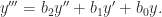


 flops and
  storage instead of the
  for some
  with
with  . It is not necessarily the case that the computed roots are the exact roots of a polynomial with coefficients
  with
with  for all
  .
.
 companion matrix as the product of two symmetric matrices. The obvious generalization of this factorization to
 denote the field
  or
or  .
. then
then  where
where  is nonsingular and
  , with each
  a companion matrix.
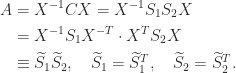
 is nonsingular, and since
  can alternatively be taken nonsingular by considering the factorization of
  , this proves a theorem of Frobenius.
 , either one of which can be taken nonsingular, such that
  .
. with the
  symmetric then
  , so
, so  is symmetric. Likewise,
  is symmetric.
 block placed on the diagonal, and he used this factorization to determine a matrix
  similar to
  it is
it is![\notag \widetilde{C} = \begin{bmatrix} a_4 & a_3 & 1 & 0 & 0 \\ 1 & 0 & 0 & 0 & 0 \\ 0 & a_2 & 0 & a_1 & 1 \\ 0 & 1 & 0 & 0 & 0 \\ 0 & 0 & 0 & a_0 & 0 \end{bmatrix} = \left[\begin{array}{cc|cc|c} a_4 & 1 & & & \\ 1 & 0 & & & \\\hline & & a_2 & 1 & \\ & & 1 & 0 & \\\hline & & & & a_0 \end{array}\right] \left[\begin{array}{c|cc|cc} 1 & & & & \\\hline & a_3 & 1 & & \\ & 1 & 0 & & \\\hline & & & a_1 & 1 \\ & & & 1 & 0 \end{array}\right].](https://s0.wp.com/latex.php?latex=%5Cnotag+%5Cwidetilde%7BC%7D+%3D+%5Cbegin%7Bbmatrix%7D++++a_4+%26+a_3+%26+1++%26+0+++%26+0++%5C%5C++++++1+%26+0+++%26+0++%26+0+++%26+0++%5C%5C++++++0+%26+a_2+%26+0++%26+a_1+%26+1++%5C%5C++++++0+%26+1+++%26+0++%26+0+++%26+0+%5C%5C++++++0+%26+0+++%26+0++%26+a_0+%26+0+%5Cend%7Bbmatrix%7D+%3D+%5Cleft%5B%5Cbegin%7Barray%7D%7Bcc%7Ccc%7Cc%7D++++a_4+%26+1+%26+++++%26+++%26+++%5C%5C++++++1+%26+0+%26+++++%26+++%26+++%5C%5C%5Chline++++++++%26+++%26+a_2+%26+1+%26+++%5C%5C++++++++%26+++%26++1++%26+0+%26+++%5C%5C%5Chline++++++++%26+++%26+++++%26+++%26++a_0+%5Cend%7Barray%7D%5Cright%5D+%5Cleft%5B%5Cbegin%7Barray%7D%7Bc%7Ccc%7Ccc%7D++++++1++%26+++++%26+++%26++++++%26+%5C%5C%5Chline+++++++++%26+a_3+%26+1+%26++++++%26+%5C%5C+++++++++%26++1++%26+0+%26++++++%26+%5C%5C%5Chline+++++++++%26+++++%26+++%26++a_1+%26+1+%5C%5C+++++++++%26+++++%26+++%26+++1++%26+0+%5Cend%7Barray%7D%5Cright%5D.+&bg=ffffff&fg=222222&s=0&c=20201002)

 of the form
 is the spectral radius of
  denotes that

 , we can set it to
  . Indeed let
  and
and  . Then
  , since
  and
and  for
for  . Furthermore, for a nonnegative matrix the spectral radius is an eigenvalue, by the Perron–Frobenius theorem, so
  is an eigenvalue of
  . Hence
  .
. satisfies
  ,
,

 is an
is an  .
.![\notag T_4 = \left[\begin{array}{@{\mskip 5mu}c*{3}{@{\mskip 15mu} r}@{\mskip 5mu}} 1 & -1 & -1 & -1 \\ & 1 & -1 & -1 \\ & & 1 & -1 \\ & & & 1 \end{array}\right], \quad T_4^{-1} = \begin{bmatrix} 1 & 1 & 2 & 4\\ & 1 & 1 & 2\\ & & 1 & 1\\ & & & 1 \end{bmatrix}.](https://s0.wp.com/latex.php?latex=%5Cnotag+++++T_4+%3D+%5Cleft%5B%5Cbegin%7Barray%7D%7B%40%7B%5Cmskip+5mu%7Dc%2A%7B3%7D%7B%40%7B%5Cmskip+15mu%7D+r%7D%40%7B%5Cmskip+5mu%7D%7D++++++1+%26+++-1++%26++-1++%26+-1+%5C%5C++++++++%26++++1++%26++-1++%26+-1+%5C%5C++++++++%26+++++++%26+++1++%26+-1+%5C%5C++++++++%26+++++++%26++++++%26++1++++++++++++%5Cend%7Barray%7D%5Cright%5D%2C+%5Cquad+++T_4%5E%7B-1%7D+%3D++++%5Cbegin%7Bbmatrix%7D++++1+%26+1+%26+2+%26+4%5C%5C+++%26+1+%26+1+%26+2%5C%5C+++%26+++%26+1+%26+1%5C%5C+++%26+++%26+++%26+1++++%5Cend%7Bbmatrix%7D.+&bg=ffffff&fg=222222&s=0&c=20201002)
 is the matrix
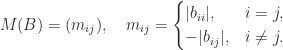

 is nonnegative we have
 can be computed in
  of an
of an 
 were to be formed explicitly.
 , which follows from
  for the
  with the same
  by
by![\notag A_4 = \left[\begin{array}{@{\mskip 5mu}c*{3}{@{\mskip 15mu} r}@{\mskip 5mu}} 2 & -1 & & \\ -1 & 2 & -1 & \\ & -1 & 2 & -1 \\ & & -1 & 2 \end{array}\right], \quad A_4^{-1} = \begin{bmatrix} \frac{4}{5} & \frac{3}{5} & \frac{2}{5} & \frac{1}{5}\\[\smallskipamount] \frac{3}{5} & \frac{6}{5} & \frac{4}{5} & \frac{2}{5}\\[\smallskipamount] \frac{2}{5} & \frac{4}{5} & \frac{6}{5} & \frac{3}{5}\\[\smallskipamount] \frac{1}{5} & \frac{2}{5} & \frac{3}{5} & \frac{4}{5} \end{bmatrix}.](https://s0.wp.com/latex.php?latex=%5Cnotag+++++A_4+%3D+%5Cleft%5B%5Cbegin%7Barray%7D%7B%40%7B%5Cmskip+5mu%7Dc%2A%7B3%7D%7B%40%7B%5Cmskip+15mu%7D+r%7D%40%7B%5Cmskip+5mu%7D%7D++++++2+%26+++-1++%26++++++%26++++%5C%5C+++++-1+%26++++2++%26++-1++%26++++%5C%5C++++++++%26++++-1+%26+++2++%26++-1+%5C%5C++++++++%26+++++++%26++-1++%26++2++++++++++++%5Cend%7Barray%7D%5Cright%5D%2C+%5Cquad+++A_4%5E%7B-1%7D+%3D++++%5Cbegin%7Bbmatrix%7D+++%5Cfrac%7B4%7D%7B5%7D+%26+%5Cfrac%7B3%7D%7B5%7D+%26+%5Cfrac%7B2%7D%7B5%7D+%26+%5Cfrac%7B1%7D%7B5%7D%5C%5C%5B%5Csmallskipamount%5D+++%5Cfrac%7B3%7D%7B5%7D+%26+%5Cfrac%7B6%7D%7B5%7D+%26+%5Cfrac%7B4%7D%7B5%7D+%26+%5Cfrac%7B2%7D%7B5%7D%5C%5C%5B%5Csmallskipamount%5D+++%5Cfrac%7B2%7D%7B5%7D+%26+%5Cfrac%7B4%7D%7B5%7D+%26+%5Cfrac%7B6%7D%7B5%7D+%26+%5Cfrac%7B3%7D%7B5%7D%5C%5C%5B%5Csmallskipamount%5D+++%5Cfrac%7B1%7D%7B5%7D+%26+%5Cfrac%7B2%7D%7B5%7D+%26+%5Cfrac%7B3%7D%7B5%7D+%26+%5Cfrac%7B4%7D%7B5%7D+%5Cend%7Bbmatrix%7D.+&bg=ffffff&fg=222222&s=0&c=20201002)
 having positive diagonal elements. However, more is true, as the next result shows.
 in which
  and
and ![\notag A = \begin{array}[b]{@{\mskip27mu}c@{\mskip-20mu}c@{\mskip-10mu}c@{}} \scriptstyle 1 & \scriptstyle n-1 & \\ \multicolumn{2}{c}{ \left[\begin{array}{c@{~}c@{~}} \alpha & b^T \\ c^T & E \\ \end{array}\right]} & \mskip-14mu\ \begin{array}{c} \scriptstyle 1 \\ \scriptstyle n-1 \end{array} \end{array}, \quad \alpha > 0, \quad b\le 0, \quad c \le 0.](https://s0.wp.com/latex.php?latex=%5Cnotag++++A+%3D++++%5Cbegin%7Barray%7D%5Bb%5D%7B%40%7B%5Cmskip27mu%7Dc%40%7B%5Cmskip-20mu%7Dc%40%7B%5Cmskip-10mu%7Dc%40%7B%7D%7D++++%5Cscriptstyle+1+%26++++%5Cscriptstyle+n-1+%26++++%5C%5C++++%5Cmulticolumn%7B2%7D%7Bc%7D%7B++++++++%5Cleft%5B%5Cbegin%7Barray%7D%7Bc%40%7B%7E%7Dc%40%7B%7E%7D%7D++++++++++++++++++%5Calpha+%26+b%5ET+%5C%5C++++++++++++++++++c%5ET++++%26+E++%5C%5C++++++++++++++%5Cend%7Barray%7D%5Cright%5D%7D++++%26+%5Cmskip-14mu%5C++++++++++%5Cbegin%7Barray%7D%7Bc%7D++++++++++++++%5Cscriptstyle+1+%5C%5C++++++++++++++%5Cscriptstyle+n-1++++++++++++++%5Cend%7Barray%7D++++%5Cend%7Barray%7D%2C+++%5Cquad+%5Calpha+%3E+0%2C+%5Cquad+b%5Cle+0%2C+%5Cquad+c+%5Cle+0.+&bg=ffffff&fg=222222&s=0&c=20201002)

 is the Schur complement of
  in
in  and the first row of
  are of the form required for a triangular
 . It is easy to see that
  , and hence Theorem
  is strictly diagonally dominant by columns for some diagonal matrix
  with
with  for all
 because of the sign pattern of
  , and partial pivoting does not require row interchanges. The effect of row scaling on LU factorization is easy to see:
 is unit lower triangular, so that
  are the LU factors of
![\notag A^{-1} = \begin{bmatrix} \displaystyle\frac{1}{\epsilon}& 0& \displaystyle\frac{1}{\epsilon}\\[\bigskipamount] \displaystyle\frac{1}{\epsilon}& 1 & \displaystyle\frac{1 + \epsilon}{\epsilon}\\[\bigskipamount] 0& 0& 1 \end{bmatrix} \ge 0,](https://s0.wp.com/latex.php?latex=%5Cnotag++A%5E%7B-1%7D+%3D++++%5Cbegin%7Bbmatrix%7D++++++++%5Cdisplaystyle%5Cfrac%7B1%7D%7B%5Cepsilon%7D%26+0%26+%5Cdisplaystyle%5Cfrac%7B1%7D%7B%5Cepsilon%7D%5C%5C%5B%5Cbigskipamount%5D++++++++%5Cdisplaystyle%5Cfrac%7B1%7D%7B%5Cepsilon%7D%26+1+%26+%5Cdisplaystyle%5Cfrac%7B1+%2B+%5Cepsilon%7D%7B%5Cepsilon%7D%5C%5C%5B%5Cbigskipamount%5D++++++++++++++++++0%26+++++++++++0%26+++++1++++%5Cend%7Bbmatrix%7D+%5Cge+0%2C+&bg=ffffff&fg=222222&s=0&c=20201002)
 element of the LU factor
  , which means that
 is large, in that the computed LU factors have a large relative residual. We conclude that pivoting is necessary for numerical stability in LU factorization of
  is based on a splitting
  with
with  . This iteration converges for all starting vectors
  if
if  . Much interest has focused on regular splittings, which are defined as ones for which
  and
and  . An
. An  ) are all convergent for
  of an
of an 
 in
in  be the transition matrix of a Markov chain. Then
  . A nonnegative vector
  such that
  is called a stationary distribution vector and is of interest for describing the properties of the Markov chain. To compute
 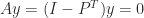 . Clearly,
  , so
, so  -matrix:
  holds for any
  Decompositions of Generalized Diagonally Dominant Matrices
 exceeds
  . Note that in some references, such as Horn and Johnson (2013), the reverse ordering is used, with
  the largest eigenvalue. When it is necessary to specify what matrix
  is an eigenvalue of we write
  : the
: the  th largest eigenvalue of
  .
. is the quadratic form
  for
for  . As
. As  , where
  is unitary and
  . Then

 , respectively, This characterization of the extremal eigenvalues of
  is due to Lord Rayleigh (John William Strutt), and
  is called a Rayleigh quotient. The intermediate eigenvalues correspond to saddle points of
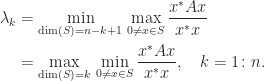
 of Hermitian matrices. However, the Courant–Fischer theorem yields the upper and lower bounds


 and
and  ,
,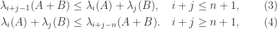
 . Inequality (3) with
  gives
gives
 , combined with (2), gives
 to the interval between two adjacent eigenvalues of
  of
of  of
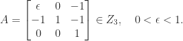
of  A specific example, in MATLAB, is
 and the trace is the sum of the eigenvalues, we can write
 are nonnegative and sum to
  , the norm of the perturbation, then most of the increase in the eigenvalues is concentrated in the largest, since (5) bounds how much the smaller eigenvalues can change:
 negative eigenvalues then (3) with
  gives
gives
 gives
gives
 , for which we have
 eigenvalues appear in one of these inequalities and
  appear in both. Therefore
  of the eigenvalues are equal to
  eigenvalues can differ from
  changes at most
  and
and  and so taking
  in (3) and
  in (4) gives
 .
.
 interlace those of
  for all
  is given in the next result.
 in the formula
  that
that  for all
  . These relations are the first and last in a sequence of inequalities relating sums of eigenvalues to sums of diagonal elements obtained by Schur in 1923.
 is the set of diagonal elements of
  .
.![[\lambda_1,\dots,\lambda_n]](https://s0.wp.com/latex.php?latex=%5B%5Clambda_1%2C%5Cdots%2C%5Clambda_n%5D&bg=ffffff&fg=222222&s=0&c=20201002) of eigenvalues majorizes the ordered vector
of eigenvalues majorizes the ordered vector ![[\widetilde{a}_{11},\dots,\widetilde{a}_{nn}]](https://s0.wp.com/latex.php?latex=%5B%5Cwidetilde%7Ba%7D_%7B11%7D%2C%5Cdots%2C%5Cwidetilde%7Ba%7D_%7Bnn%7D%5D&bg=ffffff&fg=222222&s=0&c=20201002) of diagonal elements.
of diagonal elements.
 . Here is an illustration in MATLAB.
 , the inequality is the same as the upper bound of (1), and for
  it is an equality:
  .
. , the transformation
  is a congruence transformation. Sylvester’s law of inertia says that congruence transformations preserve the inertia. A result of Ostrowski (1959) goes further by providing bounds on the ratios of the eigenvalues of the original and transformed matrices.
 and
and  ,
,
 .
. and so Ostrowski’s theorem reduces to the fact that a congruence with a unitary matrix is a similarity transformation and so preserves eigenvalues. The theorem shows that the further