April 2023 – Nick Higham

For a polynomial

$\notag \phi(t) = a_kt^k + \cdots + a_1t + a_0,$

where $a_k\in\mathbb{C}$ for all $k$ , the matrix polynomial obtained by evaluating $\phi$ at $A\in\mathbb{C}^{n \times n}$ is

$\notag \phi(A) = a_kA^k + \cdots + a_1A + a_0 I.$

(Note that the constant term is $a_0 A^0 = a_0 I$ ). The polynomial $\phi$ is monic if $a_k = 1$ .

The characteristic polynomial of a matrix 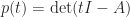$A\in\mathbb{C}^{n \times n}$ is $p(t) = \det(t I - A)$ , a degree $n$ monic polynomial whose roots are the eigenvalues of $A$ . The Cayley–Hamilton theorem tells us that $p(A) = 0$ , but $p$ may not be the polynomial of lowest degree that annihilates $A$ . The monic polynomial $\psi$ of lowest degree such that $\psi(A) = 0$ is the minimal polynomial of $A$ . Clearly, $\psi$ has degree at most $n$ .

The minimal polynomial divides any polynomial $\phi$ such that $\phi(A) = 0$ , and in particular it divides the characteristic polynomial. Indeed by polynomial long division we can write $\phi(t) = q(t)\psi(t) + r(t)$ , where the degree of $r$ is less than the degree of $\psi$ . Then

$\notag 0 = \phi(A) = q(A) \psi(A) + r(A) = r(A).$

If $r\ne 0$ then we have a contradiction to the minimality of the degree of $\psi$ . Hence $r = 0$ and so $\psi$ divides $\phi$ .

The minimal polynomial is unique. For if $\psi_1$ and $\psi_2$ are two different monic polynomials of minimum degree $m$ such that $\psi_i(A) = 0$ , $i = 1,2$ , then $\psi_3 = \psi_1 - \psi_2$ is a polynomial of degree less than $m$ and $\psi_3(A) = \psi_1(A) - \psi_2(A) = 0$ , and we can scale $\psi_3$ to be monic, so by the minimality of $m$ , $\psi_3 = 0$ , or $\psi_1 = \psi_2$ .

If $A$ has distinct eigenvalues then the characteristic polynomial and the minimal polynomial are equal. When $A$ has repeated eigenvalues the minimal polynomial can have degree less than $n$ . An extreme case is the identity matrix, for which $\psi(t) = t - 1$ , since $\psi(I) = I - I = 0$ . On the other hand, for the Jordan block

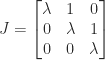
$\notag J = \begin{bmatrix} \lambda & 1 & 0 \\ 0 & \lambda & 1 \\ 0 & 0 & \lambda \end{bmatrix}$

the characteristic polynomial and the minimal polynomial are both equal to $(\lambda - 1)^3$ .

The minimal polynomial has degree less than $n$ when in the Jordan canonical form of $A$ an eigenvalue appears in more than one Jordan block. Indeed it is not hard to show that the minimal polynomial can be written

$\notag \psi(t) = \displaystyle\prod_{i=1}^s (t-\lambda_i)^{n_i},$

where $\lambda_1,\lambda_2,\dots,\lambda_s$ are the distinct eigenvalues of $A$ and $n_i$ is the dimension of the largest Jordan block in which $\lambda_i$ appears. This expression is composed of linear factors (that is, $n_i = 1$ for all $i$ ) if and only if $A$ is diagonalizable.

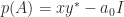
To illustrate, for the matrix

$\notag A = \left[\begin{array}{cc|c|c|c} \lambda & 1 & & & \\ & \lambda & & & \\\hline & & \lambda & & \\\hline & & & \mu & \\\hline & & & & \mu \end{array}\right]$

in Jordan form (where blank elements are zero), the minimal polynomial is $\psi(t) = (t-\lambda)^2(t-\mu)$ , while the characteristic polynomial is $p(t) = (t-\lambda)^3(t-\mu)^2$ .

What is the minimal polynomial of a rank- $1$ matrix, $A = xy^* \ne 0$ ? Since $A^2 = (y^*x) xy^*$ , we have $q(A) = 0$ for $q(t) = t^2 - (y^*x) t = t^2 - \mathrm{trace}(A) t$ . For any linear polynomial $p(t) = t - a_0$ , $p(A) = xy^* - a_0 I$ , which is nonzero since $xy^*$ has rank $1$ and $I$ has rank $n$ . Hence the minimal polynomial is $q$ .

The minimal polynomial is important in the theory of matrix functions and in the theory of Krylov subspace methods. One does not normally need to compute the minimal polynomial in practice.

Month: April 2023

What Is the Minimal Polynomial of a Matrix?

Related Blog Posts

Ten Year Anniversary of the Blog

Related Blog Posts

Share this:

Share this: