Wilkinson’s Rounding Errors Book Reprinted by SIAM

James Wilkinson’s 1963 book Rounding Errors in Algebraic Processes has been hugely influential. It came at a time when the effects of rounding errors on numerical computations in finite precision arithmetic had just starting to be understood, largely due to Wilkinson’s pioneering work over the previous two decades. The book gives a uniform treatment of error analysis of computations with polynomials and matrices and it is notable for making use of backward errors and condition numbers and thereby distinguishing problem sensitivity from the stability properties of any particular algorithm.

The book was originally published by Her Majesty’s Stationery Office in the UK and Prentice-Hall in the USA. It was reprinted by Dover in 1994 but has been out of print for some time. SIAM has now reprinted the book in its Classics in Applied Mathematics series. It is available from the SIAM Bookstore and, for those with access to it, the SIAM Institutional Book Collection.

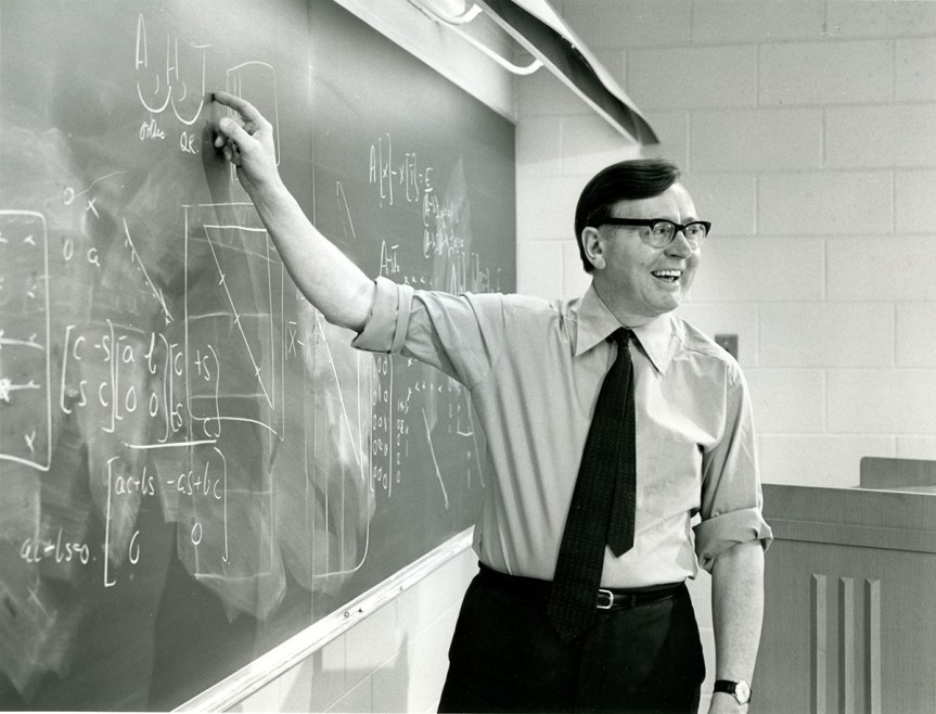
I was asked to write a foreword to the book, which I include below. The photo shows Wilkinson lecturing at Argonne National Laboratory. For more about Wilkinson see the James Hardy Wilkinson web page.

Foreword

Rounding Errors in Algebraic Processes was the first book to give detailed analyses of the effects of rounding errors on a variety of key computations involving polynomials and matrices.

The book builds on James Wilkinson’s 20 years of experience in using the ACE and DEUCE computers at the National Physical Laboratory in Teddington, just outside London. The original design for the ACE was prepared by Alan Turing in 1945, and after Turing left for Cambridge Wilkinson led the group that continued to design and build the machine and its software. The ACE made its first computations in 1950. A Cambridge educated mathematician, Wilkinson was perfectly placed to develop and analyze numerical algorithms on the ACE and the DEUCE (the commercial version of the ACE). The intimate access he had to the computers (which included the ability to observe intermediate computed quantities on lights on the console) helped Wilkinson to develop a deep understanding of the numerical methods he was using and their behavior in finite precision arithmetic.

The principal contribution of the book is the analysis of the effects of rounding errors on algorithms, using backward error analysis (then in its infancy) or forward error analysis as appropriate. The book laid the foundations for the error analysis of algebraic processes on digital computers.

Three types of computer arithmetic are analyzed: floating-point arithmetic, fixed-point arithmetic (in which numbers are represented as a number on a fixed interval such as $[-1,1]$ with a fixed scale factor), and block floating-point arithmetic, which is a hybrid of floating-point arithmetic and fixed-point arithmetic. Although floating-point arithmetic dominates today’s computational landscape, fixed-point arithmetic is widely used in digital signal processing and block floating-point arithmetic is enjoying renewed interest in machine learning.

A notable feature of the book is its careful consideration of problem sensitivity, as measured by condition numbers, and this approach inspired future generations of numerical analysis textbooks.

Wilkinson recognized that the worst-case error bounds he derived are pessimistic and he noted that more realistic bounds are obtained by taking the square roots of the dimension-dependent terms (see pages 26, 52, 102, 151). In recent years, rigorous results have been derived that support Wilkinson’s intuition: they show that bounds with the square roots of the constants hold with high probability under certain probabilistic assumptions on the rounding errors.

It is entirely fitting that Rounding Errors in Algebraic Processes is reprinted in the SIAM Classics series. The book is a true classic, it continues to be well-cited, and it will remain a valuable reference for years to come.

Handbook of Writing for the Mathematical Sciences, Third Edition

The third edition of Handbook of Writing for the Mathematical Sciences was published by SIAM in January 2020. It is SIAM’s fourth best selling book of all time if sales for the first edition (1993) and second edition (1998) are combined, and it is in my top ten most cited outputs. As well as being used by individuals from students to faculty, it is a course text on transferable skills modules in many mathematics departments. A number of publishers cite the book as a reference for recommended style—see, for example, the AMS Author Handbook, the SIAM Style Manual and, outside mathematics and computing, the Chicago Manual of Style.

Parts of the second edition were becoming out of date, as they didn’t reflect recent developments in publishing (open access publishing, DOIs, ORCID, etc.) or workflow (including modern LaTeX packages, version control, and markup languages). I’ve also learned a lot more about writing over the last twenty years.

I made a variety of improvements for the third edition. I reorganized the material in a way that is more logical and makes the book easier to use for reference. I also improved the design and formatting and checked and updated all the references.

I removed content that was outdated or is now unnecessary. For example, nowadays there is no need to talk about submitting a hard copy manuscript, or one not written in LaTeX, to a publisher. I removed the 20-page appendix Winners of Prizes for Expository Writing, since the contents can now be found on the web, and likewise for the appendix listing addresses of mathematical organizations.

I also added a substantial amount of new material. Here are some of the more notable changes.

A new chapter Workflow discusses how to organize and automate the many tasks involved in writing. With the increased role of computers in writing and the volume of digital material we produce it is important that we make efficient use of text editors, markup languages, tools for manipulating plain text, spellcheckers, version control, and much more.
The chapter on $\LaTeX$ has been greatly expanded, reflecting both the many new and useful packages and my improved knowledge of typesetting.
I used the enumitem $\LaTeX$ package to format all numbered and bulleted lists. This results in more concise lists that make better use of the page, as explained in this blog post.
I wrote a new chapter on indexing at the same time as I was reading the literature on indexing and making an improved index for the book. Indexing is an interesting task, but most of us do it only occasionally so it is hard to become proficient. This is my best index yet, and the indexing chapter explains pretty much everything I’ve learned abut the topic.
Since the second edition I have changed my mind about how to typeset tables. I am now a convert to minimizing the use of rules and to using the booktabs $\LaTeX$ package, as explained in this blog post.
The chapter Writing a Talk now illustrates the use of the Beamer $\LaTeX$ package.
The book uses color for syntax highlighted $\LaTeX$ listings and examples of slides.
Sidebars in gray boxes give brief diversions on topics related to the text, including several on “Publication Peculiarities”.
An expanded chapter English Usage includes new sections on Zombie Nouns; Double Negatives; Serial, or Oxford, Comma; and Split Infinitives.
There are new chapters on Writing a Blog Post; Refereeing and Reviewing; Writing a Book; and, as discussed above, Preparing an Index and Workflow.
The bibliography now uses the backref $\LaTeX$ package to point back to the pages on which entries are cited, hence I removed the author index.
As well as updating the bibliography I have added DOIs and URL links, which can be found in the online version of the bibliography in bbl and PDF form, which is available from the book’s website.

At 353 pages, and allowing for the appendices removed and the more efficient formatting, the third edition is over 30 percent longer than the second edition.

As always, working with the SIAM staff on the book was a pleasure. A special thanks goes to Sam Clark of T&T Productions, who copy edited the book. Sam, with whom I have worked on two previous book projects, not only edited for SIAM style but found a large number of improvements to the text and showed me some things I did not know about $\LaTeX$ .

SIAM News has published an interview with me about the book and mathematical writing and publishing.

Here is a word cloud for the book, generated in MATLAB using the wordcloud function, based on words of 6 or more characters.

A Mathematician Looks at the Collins English Dictionary

I have several dictionaries on my shelf, among which is a well-thumbed Collins English Dictionary (third edition, 1991). Earlier this year I acquired the thirteenth edition (2018). At 26.5cm high, 20cm wide, and 6.5cm deep, and weighing approximately 2.5kg, it’s an imposing tome. It’s printed on thin paper with minimal show-through and in a specially designed font (Collins Fedra) that is very legible.

The thirteenth edition, which I will abbreviate to CED13, is a wonderful acquisition for any dictionary lover. It has a wide coverage, including

new words such as micromort (“a unit of risk equal to a one-in-a million chance of dying”),
obscure words such as compotation (“the act of drinking together in a company”), and
a wide selection of proper nouns, including my home town Eccles and, somewhat unexpectedly, Laurel and Hardy and Torvill and Dean (Olympic ice dance champions, 1984).

It has no appendices on English usage, mathematical symbols, chemical elements, etc., as are found in many dictionaries—which is fine with me as I rarely use them.

I decided to take a close look at some of the mathematical words in the CED.

“determinant n maths: a square array of elements that represents the sum of certain products of these elements, used to solve simultaneous equations, in vector studies, etc.”

This definition has two problems. First, a determinant is the sum, not something that represents the sum. Of, course, one will find in some textbooks statements such as “swapping two rows of a determinant changes its sign”, but it’s odd that this informal usage of determinant as array is the only one mentioned. A second problem is that the determinant is not a sum of products: it is a signed sum of products and it is the permanent (not in this dictionary) that is obtained by taking all positive signs.

“matrix n maths a rectangular array of elements set out in rows and columns, used to facilitate the solution of problems, such as transformation of coordinates.”

A matrix is more than just an array: its key characteristic is that it has algebraic operations defined on it.

“rounding: n computing a process in which a number is approximated as the closest number that can be expressed using the number of bits or digits available.”

Rounding is not specifically a computing term—it’s more fundamentally a mathematical operation and predates computing. Bits are special cases of digits. And rounding does not have to be to the closest number: in some situations once needs to round to the next larger or smaller number.

“index n maths c a subscript or superscript to the right of a variable to express a set of variables, as in using $x_i$ for $x_1$ , $x_2$ , $x_3$ , etc”

An index does not (except maybe in informal usage) express a set, but rather identifies a member of a set.

“supercomputer n a powerful computer that can process large quantities of data of a similar type very quickly.”

Supercomputers do mathematical calculations (and are ranked on their speed in doing so), which is not apparent from this definition. I’m also not sure why “of a similar type” is necessary. The PC on which I am typing is a supercomputer according to this definition!

“integral n maths the limit of an increasingly large number of increasingly smaller quantities, related to the function that is being integrated (the integrand). The independent variables may be confined within certain limits (definite integral) or in the absence of limits (indefinite integral).”

This seems to be an attempt to state informally the Riemann sum definition of definite integration. Sadly, it’s technically incomplete and sure to baffle anyone who doesn’t already know about Riemann sums. It would have been much better to simply say that integration is the inverse of differentiation. The second sentence is grammatically incorrect.

“fractal maths n a figure or surface generated by successive subdivisions of a simpler polygon or polyhedron, according to some iterative process.”

Surely any definition should mention fractional dimension and self-similarity? This definition excludes the fractal that is the boundary of the Mandelbrot set.

I’m not too surprised by these weaknesses, because in 1994 I wrote an article Which Dictionary for the Mathematical Scientist? (PDF file here) in which I evaluated several dictionaries (including CED3) from the point of view of their mathematical words and found problems such as those above in several of them.

Despite these criticisms, I very much like this dictionary and I use it as much as the other dictionaries on my desk. It is especially good on the computing side. I was pleased to see that my favourite editor, emacs, is included (though I’m not sure why it is not capitalized). Vi users will be sad to hear that Vi is not included. A good number of programming languages are present, including awk (uncapitalized), Java, and Javascript, but not, C++ (how would that be alphabetized?), Python, or R.

A particularly notable definition is

“flops or FLOPS n acronym for floating-point operations per second: used as a measure of computer processing power (in combination with a prefix): megaflops; gigaflops.”

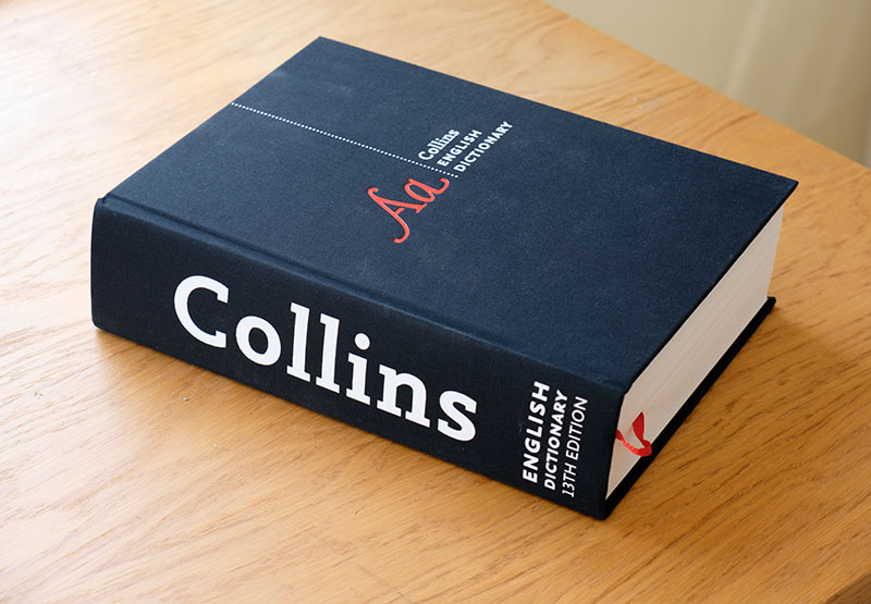
This is much better than the Oxford English Dictionary’s definition of the singular flop as “a floating-point operation per second”. There are also entries for petaflop, “ $10^{15}$ floating-point operations a second”, and teraflop, “a thousand billion floating-point operations a second”. I just wish the latter definition contained “ $10^{12}$ “, because there is scope for misunderstanding because of the alternative meaning of a billion as a million million in the UK.

Foundations of Applied Mathematics Book Series

Foundations of Applied Mathematics, Volume 1: Mathematical Analysis was published by SIAM this summer. Written by Jeffrey Humpherys, Tyler J. Jarvis, and Emily J. Evans, all from Brigham Young University, this is the first of a four-book series, aimed at the upper undergraduate or first year graduate level. It lays the analysis and linear algebra foundations that the authors feel are needed for modern applied mathematics.

The next book, Volume 2: Algorithms, Approximation, and Optimization, is scheduled for publication in 2018.

At 689 pages, hardback, beautifully typeset on high quality paper, and with four colours used for the diagrams and boxed text, this is a physically impressive book. Unusually for a SIAM book, it contains a dust jacket. I got a surprise when I took it off: underneath is a front cover very different to the dust jacket, containing a huge number 1. I like it and am leaving my book cover-free.

I always look to see what style decisions authors have made, as I ponder them a lot when writing my own books. One was immediately obvious: the preface uses five Oxford commas in the first six sentences!

I have only had time to dip into a few parts of the book, so this is not a review. But here are some interesting features.

Chapter 15, Rings and Polynomials, covers a lot of ground under this general framework, including the Euclidean algorithm, the Lagrange and Newton forms of the polynomial interpolant, the Chinese remainder theorem (of which several applications are mentioned), and partial fractions. This chapter has attracted a lot of interest on Reddit.
The authors say in the preface that one of their biggest innovations is treating spectral theory using the Dunford-Schwartz approach via resolvents.
There is a wealth of support material available here. More material is available here.

It’s great to see such an ambitious project, especially with SIAM as the publisher. If you are teaching applied mathematics with a computational flavour you should check it out.

A Second Course in Linear Algebra, by Garcia and Horn (2017)

The publication of a new linear algebra textbook is not normally a cause for excitement. However, Roger Horn is co-author of two of the most highly regarded and widely used books on matrix analysis: Matrix Analysis (2nd edition, 2013) and Topics in Matrix Analysis (1991), both co-authored with Charles Johnson. It is therefore to be expected that this new book by Garcia and Horn will offer something special.

Chapter 0 (Preliminaries) summarizes basic concepts and definitions, often stating results without proof (for example, properties of determinants). Chapters 1 (Vector Spaces) and 2 (Bases and Similarity) are described as reviews, but give results with proofs and examples. The second course proper starts with Chapter 3 (Block Matrices). As the chapter title suggests, the book makes systematic use of block matrices to simplify the treatment, and it is very much based on matrices rather than linear transformations.

Two things stand out about this book. First, it lies part-way between a traditional linear algebra text and texts with a numerical linear algebra focus. Thus it includes Householder matrices (but not Givens matrices), QR factorization, and Cholesky factorization. The construction given for QR factorization is essentially the Householder QR factorization, but the existence proof for Cholesky goes via the QR factor of the Hermitian positive definite square root, rather than by constructing the Cholesky factor explicitly via the usual recurrences. The existence of square roots of Hermitian positive definite matrices is proved via the spectral decomposition. It is possible to prove the existence of square roots without using the spectral theorem, and it would have been nice to mention this, at least in an exercise.

The second impressive aspect of the book is the wide, and often quite advanced, range of topics covered, which includes polar decomposition, interlacing results for the eigenvalues of Hermitian matrices, and circulant matrices. Not covered are, for example, Perron–Frobenius theory, the power method, and functions of nonsymmetric matrices (though various special cases are covered, such as the square root of Jordan block, often in the problems). New to me are the QS decomposition of a unitary matrix, Shoda’s theorem on commutators, and the Fuglede–Putnam theorem on normal matrices.

The 16-page index occupies 3.7 percent of the book, which, according to the length criteria discussed in my article A Call for Better Indexes, is unusually thorough. However, there is some over-indexing. For example, the entry permutation consists of 7 subentries all referring to page 10, but “permutation, 10” would have sufficed. An index entry “Cecil Sagehen” puzzled me. It has two page locators: one on which that term does not appear and one for a problem beginning “Cecil Sagehen is either happy or sad”. A little investigation revealed that “Cecil the Sagehen” is the mascot of Pomona College, which is the home institution of the first author.

There is a large collection of problems that go well beyond simple illustration and computation, and it is good to see that the problems are indexed.

Here are some other observations.

The singular value decomposition (SVD) is proved via the eigensystem of $A^*A$ . Personally, I prefer the more elegant, if less intuitively obvious, proof in Golub and Van Loan’s Matrix Computations.
The treatment of Gershgorin’s theorem occupies six pages, but it omits the practically important result that if $k$ discs form a connected region that is isolated from the other discs then that region contains precisely $k$ eigenvalues.
The Cayley-Hamilton theorem is proved by using the Schur form. I would do it either via the minimal polynomial or the Jordan form, but these concepts are introduced only in later chapters.
Correlation matrices are mentioned in the preface, but do not appear in the book. They can make excellent examples.
The real Schur decomposition is not included, but rather just the special case for a real matrix having only real eigenvalues.
Matrix norms are not treated. The Frobenius norm is defined as an inner product norm and, unusually, the 2-norm is defined as the largest singular value of a matrix. There are no index entries for “matrix norm”, “norm, matrix”, “vector norm”, or “norm, vector”.
The pseudoinverse of a matrix is defined via the SVD. The Moore-Penrose conditions are not explicitly mentioned.
Three pages at the front summarize the notation and point to where terms are defined. Ironically, the oft-used notation $M_n$ for an $n \times n$ matrix, is not included.
Applications are mentioned only in passing. However, this does keep the book down to a relatively slim 426 pages.

Just as for numerical analysis texts, there will probably never exist a perfect linear algebra text.

The book is very well written and typeset. With its original presentation and choice of content it must be a strong contender for use on any second (or third) course on linear algebra. It can also serve as a reference on matrix theory: look here first and turn to Horn and Johnson if you don’t find what you want. Indeed a surprising amount of material from Horn and Johnson’s books is actually covered, albeit usually in less general form.

SIAM Books Available Worldwide from Eurospan

SIAM books are now available to individuals, bookstores, and other retailers outside North America from Eurospan, who have taken over the role previously carried out by Cambridge University Press.

This is significant news for those of us outside North America for two reasons.

Shipping is free, anywhere in the world.
SIAM members get a 30 percent discount on entering a special code at checkout. This code was emailed to all SIAM members in March 2017. If you are a SIAM member and do not have the code, you can get it by contacting SIAM customer service at siambooks@siam.org.

Check out the landing page for SIAM books at the Eurospan website.

SIAM members outside North America now have three options for ordering SIAM books.

Eurospan: 30 percent member discount; pay in GBP in the UK, euros in Europe, Australian dollars in Australian territories, US dollars everywhere else; free shipping.
SIAM Bookstore: 30 percent member discount; pay in US dollars; free shipping (at least for the near future).
Amazon: unpredictable, sometimes very small, discount; pay in currency of the particular site.

Preparing CMYK Figures for Book Printing

All printing is done in CMYK, the color space based on the four colors cyan, magenta, yellow, and black. Figures that we generate in MATLAB and other systems are invariably saved in RGB format (red, green, blue). When we send a paper for publication we submit RGB figures and they are transformed to CMYK somewhere in the production process, usually without us realizing that it has been done.

If you are one of those people who writes books and prefers to generate the final PDF yourself then you will need to convert any color figures to CMYK. The generation and use of CMYK files is something of a dark art. Here I report what I found out about it when producing the third edition (2017) of MATLAB Guide, co-authored with Des Higham. This is the first edition of the book to use color.

CMYK produces a different range of colors than RGB. Since it is a subtractive color space, designed for inks, it cannot produce some of the brilliant colors that RGB can, especially in the blues. In other words, some RGB colors are out of gamut in CMYK. (Less importantly, the converse is true: some CMYK colors cannot be produced in RGB.) This is something we are used to, but usually do not notice. Whenever we print a document on a laser printer we view a CMYK representation of the colors. In many cases, a figure will look very similar in print and on screen, but there are plenty of exceptions.

The following image shows an RGB image on the left, the result of converting that image to CMYK and then back to RGB in the middle, and a scan of a laser printer’s reproduction of the RGB image on the right. The differences between the RGB version and the other two versions may be shocking! Fortunately, when the CMYK version is viewed on a printed page in isolation from the RGB version (necessarily displayed on a monitor) it does not look so bad. [Of course, if you are reading a printed version of this post then the first two images will look essentially the same.]

After some experimentation, I settled on the following procedure, which I describe for a PDF workflow. For a PostScript workflow, PDF files need to be replaced by EPS files.

Print the whole document from an RGB file.
Find figures that look very different in print than on screen and select from those any where the difference is not acceptable. In most cases an unacceptable difference will be one where contrast between colors, or saturation of colors, has been reduced.
Edit the selected figures in Photoshop, or some other image manipulation package that can save in CMYK form, in order to produce a better looking CMYK file. In Photoshop, Image-Mode-CMYK Color converts an image to CMYK form, but before using this command you should set the correct CMYK working space under Edit-Color Settings (see the Color Space section below). You can edit the RGB image (making use of View-Proof Color to see how the image will look in CMYK, and View-Gamut Warning to see colors that will be out of gamut in CMYK) and then convert to CMYK, or you can convert to CMYK and then edit the file. Save the CMYK image as a PDF file.
Generate the PDF file of the book using the edited CMYK figures and the RGB forms of all the other figures, that is, those that did not need special treatment.
Load the PDF file into Adobe Acrobat Pro and issue the command
```
Tools - Print Production - Convert Colors
```
This converts all objects in the file to CMYK.

Of the well over 100 figures in MATLAB Guide, only two needed special treatment.

However, there was one problem with this procedure. A handful of images are screen dumps that show a MATLAB window, and these are necessarily low resolution, at 72dpi. When converted to CMYK in Adobe Acrobat these images degraded badly. The solution was to resample the images to 150dpi in Photoshop via Image-Image Size and save to PDF; conversion in Acrobat then worked fine. (Such resampling is probably good practice anyway.)

This is not quite the full story. Here are some more gory details, which are worth reading if you are actually producing a book.

Color Spaces

There is no unique CMYK or RGB color space: these spaces are device dependent. RGB spaces can have different white points and CMYK spaces are designed for particular combinations of paper and ink. Adobe Acrobat Pro offers “U.S. Web Coated (SWOP) v2”, “Uncoated FOGRA29 (ISO 12647-2:2004)” and many other inscrutably named CMYK profiles. So “convert to CMYK” is an ill-defined instruction unless the precise profile is specified. The conversion settings I used are shown in this screen dump of the dialog box, and were provided by the company who printed the book. Your settings might need to be different. 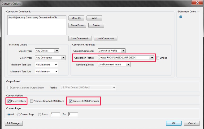There are a couple of things to note. First, Adobe Acrobat does not remember the settings in the dialog box, so they need to be re-entered every time. Second, since “Embed profile” is not selected with the settings shown, there is no way to tell which profile has been used once the conversion has been done.

Does it really matter what CMYK profile you use? Yes, if you want the best possible results. Consider the following figure. On the left is the result of converting the original RGB image to “U.S. Web Coated (SWOP) v2” and on the right is the result of converting to “Photoshop 5 default CMYK” (and converting back to RGB in both cases, the latter conversion producing no visual difference in Photoshop). There is a significant difference between the two conversions in every color except white! In principle, both conversions will produce the same result when printed with the target ink and paper, but if you choose the profile without knowing the target you have little idea what the printed result will be.

Photography Books

An important assumption in the process described above is that the accuracy of the color reproduction is not vital. For photography books this assumption clearly does not hold and conversion to CMYK enters a new and frightening realm where images might need to be individually fine-tuned. Indeed high quality photography books typically undergo one or more proof stages using actual galley proofs from the ultimate printing device, sometimes with the author present at the printing press.

Generating CMYK Files in MATLAB

Most of the figures in MATLAB Guide are (naturally) produced in MATLAB. Figures saved with the print function are by default in RGB mode. CMYK is supported for EPS and PS files only, using the ‘-cmyk’ option. This is not very useful if you are using a PDF workflow, as I do.

Instead of using the print function I experimented with export_fig, which is available on MathWorks File Exchange and can save in CMYK format to PDF, EPS, or TIFF files. export_fig creates a PDF file via an EPS file using Ghostscript.

This sounds straightforward, but I found that many of the PDF files generated by export_fig were not fully in CMYK Mode. A PDF file can contain objects in different color spaces and I had files where a color plot was in CMYK but the colorbar was in RGB! The question arises of how one can check whether a given PDF file has any RGB objects. Unfortunately, there seems to be no simple way to do so in Adobe Acrobat Pro. What one can do is invoke

Tools - Print Production - Preflight - PDF analysis - 
List objects using ICCbased CMYK - Analyze

then open up

Overview - color spaces

(I am using Adobe Acrobat Pro XI, 11.0.18; usage could differ in other versions). This should contain “DeviceCMYK color space”, but if it contains “DeviceRGB color space” or “DeviceGray color space” then RGB or Grayscale objects are present. If the latter terms appear in a multi-page PDF file, double clicking on the corresponding icon should take you to the last such object.

You can also open up

Overview - Images

to get a list of pages and object types on those pages. Double clicking on a page icon takes you to that page.

MATLAB Guide, Third Edition (2017)

The third edition of MATLAB Guide, which I co-wrote with Des Higham, has just been published by SIAM. It is a major update of the second edition (2005) to reflect the many changes in MATLAB over the last twelve years, and is 25 percent longer. There are new sections and chapters, and almost every page has changed.

The new chapters are

Object-Oriented Programming: presents an introduction to object-oriented programming in MATLAB through two examples of classes.
Graphs: describes the new MATLAB classes graph and digraph for representing and manipulating undirected graphs and directed graphs.
Large Data Sets: describes MATLAB features for handling data sets so large that they do not fit into the memory of the computer.
The Parallel Computing Toolbox: describes this widely used and increasingly important toolbox.

The chapter The Symbolic Math Toolbox has been revised to reflect the change of the underlying symbolic engine from Maple (at the time of the second edition) to MuPAD.

New sections include Empty Matrices, Matrix Properties, Argument Checking and Parsing, Fine Tuning the Display of Arrays, Live Editor, Unit Tests, String Arrays, Categorical Arrays, Tables and Timetables, and Timing Code.

Two other big changes are that figures are now printed in color and there are thirteen “Asides”, highlighted in gray boxes, which contain discussions of MATLAB-related topics, such as anonymous functions, reproducibility, and color maps.

The book was launched with a reception hosted by The Mathworks and SIAM at the SIAM booth at the Joint Mathematics Meetings in Atlanta on January 6, 2017. Jim Rundquist (Senior Education Technical Evangelist) represented MathWorks, and several SIAM staff, including SIAM Publisher David Marshall, were present.

Two delicious cakes, one containing a representation of the cover of the book, were enjoyed by reception attendees. Inspired by MATLAB, the cakes were served using slice, deal, and input, and an occasional reshape or rotate, with a pool of workers consuming them asynchronously.

Elizabeth Greenspan (Executive Editor, SIAM), Jim Rundquist (Senior Education Technical Evangelist, The MathWorks), Nick Higham (University of Manchester), Bruce Bailey (Book Marketing Associate, SIAM), and David Marshall (SIAM Publisher).

Second Edition (2016) of Learning LaTeX by David Griffiths and Des Higham

What is the best way to learn $\LaTeX$ ? Many free online resources are available, including “getting started” guides, FAQs, references, Wikis, and so on. But in my view you can’t beat using a (physical) book. A book can be read anywhere. You can write notes in it, stick page markers on it, and quickly browse it or look something up in the index.

The first edition of Learning $\LaTeX$ (1997) is a popular introduction to $\LaTeX$ characterized by its brevity, its approach of teaching by example, and its humour. (Full disclosure: the second author is my brother.)

The second edition of the book is 25 percent longer than the first and has several key additions. The amsmath package, particularly of interest for its environments for typesetting multiline equations, is now described. I often struggle to remember the differences between align, alignat, gather, and multline, but three pages of concise examples explain these environments very clearly.

The book now reflects the modern PDF workflow, based on pdflatex as the $\TeX$ engine. If you are still generating dvi files you should consider making the switch!

Other features new to this edition are a section on making bibliographies with Bib $\TeX$ and appendices on making slides with Beamer and posters with the a0poster class, both illustrated with complete sample documents.

Importantly for a book to be used for reference, there is an excellent 10.5-page index which, at about 10% of the length of the book, is unusually thorough (see the discussion on index length in my A Call for Better Indexes).

The 1997 first edition was reviewed in TUGboat (the journal of the TeX Users Group) in 2013 by Boris Veytsman, who had only just become aware of the book. He says

When Karl Berry and I discussed the current situation with $\LaTeX$ books for beginners, he mentioned the old text by Grffiths and Higham as an example of the one made “right”…

This is indeed an incredibly good introduction to $\LaTeX$ . Even today, when many good books are available for beginners, this one stands out.

No doubt Berry and Veytsman would be even more impressed by the improved and expanded second edition.

Given that I regard myself as an advanced $\LaTeX$ user I was surprised to learn something I didn’t know from the book, namely that in an \includegraphics command it is not necessary to specify the extension of the file being included. If you write \includegraphics{myfig} then pdflatex will search for myfig.png, myfig.pdf, myfig.jpg, and myfig.eps, in that order. If you specify

\DeclareGraphicsExtensions{.pdf,.png,.jpg}

in the preamble, $\LaTeX$ will search for the given extensions in the specified order. I usually save my figures in PDF form, but sometimes a MATLAB figure saved as a jpeg file is much smaller.

This major update of the first edition is beautifully typeset, printed on high quality, bright white paper, and weighs just 280g. It is an excellent guide for those new to $\LaTeX$ and a useful reference for experienced users.

Five Books on Applied Mathematics

The website Five Books consists of interviews with experts about their five favourite books in their subject. I was recently interviewed about my favourite popular applied mathematics books.

After making my original choice of books (ones that I use in my research) I realized that it was pitched at too high a level for a general audience. Identifying my revised choice was not easy, as I wanted to select books that contain a significant applied mathematics content, yet most books at the popular level are focused on pure mathematics.

I thought it would be good to include a book about equations. There are several such books, including It Must be Beautiful: Great Equations of Modern Science (2003) and The Great Equations: Breakthroughs in Science from Pythagoras to Heisenberg (2009). I chose Ian Stewart’s Seventeen Equations that Changed the World (2012), which has a strong applied mathematics slant.

After we did the interview, I saw an interview with Ian Stewart in Chalkdust magazine (a mathematics magazine produced by students at UCL), in which he said that the Seventeen Equations book is his favourite of all the books he’s written!

If you are wondering how to write a popular mathematics book, Ian gives some of the secrets in his article “How to Write a General Interest Mathematics Book” in The Princeton Companion to Applied Mathematics.

The complete set of Five Books interviews about mathematics is here.

Foreword

Share this:

Share this:

Share this:

Share this:

Share this:

Share this:

Color Spaces

Photography Books

Generating CMYK Files in MATLAB

Share this:

Share this:

Share this:

Share this: