An LU factorization of an 


![\notag \left[\begin{array}{rrrr} 3 & -1 & 1 & 1\\ -1 & 3 & 1 & -1\\ -1 & -1 & 3 & 1\\ 1 & 1 & 1 & 3 \end{array}\right] = \left[\begin{array}{rrrr} 1 & 0 & 0 & 0\\ -\frac{1}{3} & 1 & 0 & 0\\ -\frac{1}{3} & -\frac{1}{2} & 1 & 0\\ \frac{1}{3} & \frac{1}{2} & 0 & 1 \end{array}\right] \left[\begin{array}{rrrr} 3 & -1 & 1 & 1\\ 0 & \frac{8}{3} & \frac{4}{3} & -\frac{2}{3}\\ 0 & 0 & 4 & 1\\ 0 & 0 & 0 & 3 \end{array}\right]. \qquad (1)](https://s0.wp.com/latex.php?latex=%5Cnotag++++%5Cleft%5B%5Cbegin%7Barray%7D%7Brrrr%7D++++++3+%26+-1+%26+1+%26+1%5C%5C+++++-1+%26+3+%26+1+%26+-1%5C%5C+++++-1+%26+-1+%26+3+%26+1%5C%5C++++++1+%26+1+%26+1+%26+3++++%5Cend%7Barray%7D%5Cright%5D+++%3D++++%5Cleft%5B%5Cbegin%7Barray%7D%7Brrrr%7D+++++1+%26+0+%26+0+%26+0%5C%5C++++-%5Cfrac%7B1%7D%7B3%7D+%26+1+%26+0+%26+0%5C%5C++++-%5Cfrac%7B1%7D%7B3%7D+%26+-%5Cfrac%7B1%7D%7B2%7D+%26+1+%26+0%5C%5C+++++%5Cfrac%7B1%7D%7B3%7D+%26+%5Cfrac%7B1%7D%7B2%7D+%26+0+%26+1++++%5Cend%7Barray%7D%5Cright%5D++++%5Cleft%5B%5Cbegin%7Barray%7D%7Brrrr%7D++++3+%26+-1+%26+1+%26+1%5C%5C++++0+%26+%5Cfrac%7B8%7D%7B3%7D+%26+%5Cfrac%7B4%7D%7B3%7D+%26+-%5Cfrac%7B2%7D%7B3%7D%5C%5C++++0+%26+0+%26+4+%26+1%5C%5C++++0+%26+0+%26+0+%26+3++++%5Cend%7Barray%7D%5Cright%5D.+%5Cqquad+%281%29+&bg=ffffff&fg=222222&s=0&c=20201002)
An LU factorization simplifies the solution of many problems associated with linear systems. In particular, solving a linear system 


For a given 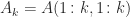

Theorem 1. The matrix
has a unique LU factorization if and only if
is nonsingular for
. If
then the factorization may exist, but if so it is not unique.
Note that the (non)singularity of 


Equating leading principal submatrices in 


![\notag \begin{aligned} \ell_{ij} &= \frac{ \det\bigl( A( [1:j-1, \, i], 1:j ) \bigr) }{ \det( A_j ) }, \quad i > j, \\ u_{ij} &= \frac{ \det\bigl( A( 1:i, [1:i-1, \, j] ) \bigr) } { \det( A_{i-1} ) }, \quad i \le j. \end{aligned}](https://s0.wp.com/latex.php?latex=%5Cnotag++++%5Cbegin%7Baligned%7D++++%5Cell_%7Bij%7D+%26%3D+%5Cfrac%7B+%5Cdet%5Cbigl%28+A%28+%5B1%3Aj-1%2C+%5C%2C+i%5D%2C+1%3Aj+%29+%5Cbigr%29+%7D%7B+%5Cdet%28+A_j+%29+%7D%2C+++++++++++++%5Cquad+i+%3E+j%2C+%5C%5C++++u_%7Bij%7D+%26%3D+%5Cfrac%7B+%5Cdet%5Cbigl%28+A%28+1%3Ai%2C+%5B1%3Ai-1%2C+%5C%2C+j%5D+%29+%5Cbigr%29+%7D+++++++++++++++++++%7B+%5Cdet%28+A_%7Bi-1%7D+%29+%7D%2C+++++++++++++%5Cquad+i+%5Cle+j.++++%5Cend%7Baligned%7D+&bg=ffffff&fg=222222&s=0&c=20201002)
Here, 


Relation with Gaussian Elimination
LU factorization is intimately connected with Gaussian elimination. Recall that Gaussian elimination transforms a matrix 


where the quantities 


The matrix factorization viewpoint is well established as a powerful paradigm for thinking and computing. Separating the computation of LU factorization from its application is beneficial. For example, given 


Computation
An LU factorization can be computed by directly solving for the components of 

Given the equivalence between LU factorization and Gaussian elimination we can also employ the Gaussian elimination equations:

This 

The 


Schur Complements
For 

The 


The first row and column of 


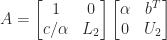
is an LU factorization of
For several matrix structures it is immediate that 


- symmetric positive definite matrices,
-matrices,
- matrices (block) diagonally dominant by rows or columns.
(The proofs of these properties are nontrivial.) Note that the matrix (1) is row diagonally dominant, as is its
We say that 


Theorem 2. Let
Proof. In (2), the first column of
and
have only
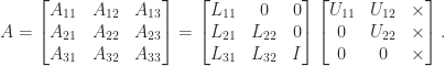
Block Implementations
In order to achieve high performance on modern computers with their hierarchical memories, LU factorization is implemented in a block form expressed in terms of matrix multiplication and the solution of multiple right-hand side triangular systems. We describe two block forms of LU factorization. First, consider a block form of (2) with block size 


Here, 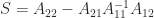
- Factor
.
- Solve
for
.
- Solve
for
.
- Form
.
- Repeat steps 1–4 on
.
The factorization on step 1 can be done by any form of LU factorization. This algorithm is known as a right-looking algorithm, since it accesses data to the right of the block being worked on (in particular, at each stage lines 2 and 4 access the last few columns of the matrix).
An alternative algorithm can derived by considering a block 
We now compute the middle block column of
- Solve
- Factor
.
- Solve
for
.
- Repartition so that the first two block columns become a single block column and repeat steps 1–4.
This algorithm corresponds to the
Our description of these block algorithms emphasizes the mathematical ideas. The implementation details, especially for the left-looking algorithm, are not trivial. The optimal choice of block size 

An important point is that all these different forms of LU factorization, no matter which
Rectangular Matrices
Although it is most commonly used for square matrices, LU factorization is defined for rectangular matrices, too. If 


Block LU Factorization
Another form of LU factorization relaxes the structure of
Note that
An example of a block LU factorization is
![\notag A = \left[ \begin{array}{rr|rr} 0 & 1 & 1 & 1 \\ -1 & 1 & 1 & 1 \\\hline -2 & 3 & 4 & 2 \\ -1 & 2 & 1 & 3 \\ \end{array} \right] = \left[ \begin{array}{cc|cc} 1 & 0 & 0 & 0 \\ 0 & 1 & 0 & 0 \\\hline 1 & 2 & 1 & 0 \\ 1 & 1 & 0 & 1 \\ \end{array} \right] \left[ \begin{array}{rr|rr} 0 & 1 & 1 & 1 \\ -1 & 1 & 1 & 1 \\\hline 0 & 0 & 1 & -1 \\ 0 & 0 & -1 & 1 \\ \end{array} \right].](https://s0.wp.com/latex.php?latex=%5Cnotag+++++A+%3D++++++%5Cleft%5B+%5Cbegin%7Barray%7D%7Brr%7Crr%7D++++++0++%26++1++%26++1++%26++1++%5C%5C+++++-1++%26++1++%26++1++%26++1++%5C%5C%5Chline+++++-2++%26++3++%26++4++%26++2++%5C%5C+++++-1++%26++2++%26++1++%26++3++%5C%5C+++++++++++++%5Cend%7Barray%7D++++++%5Cright%5D++++++%3D++++++%5Cleft%5B+%5Cbegin%7Barray%7D%7Bcc%7Ccc%7D++++++1++%26++0++%26++0++%26++0++%5C%5C++++++0++%26++1++%26++0++%26++0++%5C%5C%5Chline++++++1++%26++2++%26++1++%26++0++%5C%5C++++++1++%26++1++%26++0++%26++1++%5C%5C+++++++++++++%5Cend%7Barray%7D++++++%5Cright%5D++++++%5Cleft%5B+%5Cbegin%7Barray%7D%7Brr%7Crr%7D++++++0++%26++1++%26++1++%26++1++%5C%5C+++++-1++%26++1++%26++1++%26++1++%5C%5C%5Chline++++++0++%26++0++%26++1++%26+-1++%5C%5C++++++0++%26++0++%26+-1++%26++1++%5C%5C+++++++++++++%5Cend%7Barray%7D++++++%5Cright%5D.+&bg=ffffff&fg=222222&s=0&c=20201002)
LU factorization fails on 


Conditions for the existence of a block LU factorization are analogous to, but less stringent than, those for LU factorization in Theorem 1.
Theorem 3. The matrix
leading principal block submatrices of
The conditions in Theorem 3 can be shown to be satisfied if
Note that to solve a linear system 
Sensitivity
If 


Since 


where 

Pivoting and Numerical Stability
Since not all matrices have an LU factorization, we need the option of applying row and column interchanges to ensure that the pivots are nonzero unless the column in question is already in triangular form.
In finite precision computation it is important that computed LU factors 


See What Is the Growth Factor for Gaussian Elimination? for details of pivoting strategies and see Randsvd Matrices with Large Growth Factors for some recent research on growth factors.
References
This is a minimal set of references, which contain further useful references within.
- Jack J. Dongarra, Iain S. Duff, Danny C. Sorensen, and Henk A. Van der Vorst, Numerical Linear Algebra for High-Performance Computers, Society for Industrial and Applied Mathematics, Philadelphia, PA, USA, 1998. (For different implementations of LU factorization.)
- Nicholas J. Higham, Accuracy and Stability of Numerical Algorithms, second edition, Society for Industrial and Applied Mathematics, Philadelphia, PA, USA, 2002.
Related Blog Posts
- Randsvd Matrices with Large Growth Factors (2020)
- What Is a Block Matrix? (2020)
- What is a Diagonally Dominant Matrix? (2021)
- What Is the Growth Factor for Gaussian Elimination? (2020)
This article is part of the “What Is” series, available from https://nhigham.com/category/what-is and in PDF form from the GitHub repository https://github.com/higham/what-is.
