What Is the Perron–Frobenius Theorem?

A real matrix is nonnegative if all its elements are nonnegative and it is positive if all its elements are positive. Nonnegative matrices arise in a wide variety of applications, for example as matrices of probabilities in Markov processes and as adjacency matrices of graphs. Information about the eigensystem is often essential in these applications.

Perron (1907) proved results about the eigensystem of a positive matrix and Frobenius (1912) extended them to nonnegative matrices.

The following three results of increasing specificity summarize the key spectral properties of nonnegative matrices proved by Perron and Frobenius. Recall that a simple eigenvalue of an $n\times n$ matrix is one with algebraic multiplicity $1$ , that is, it occurs only once in the set of $n$ eigenvalues. We denote by $\rho(A)$ the spectral radius of $A$ , the largest absolute value of any eigenvalue of $A$ .

Theorem 1. (Perron–Frobenius) If $A\in\mathbb{R}^{n\times n}$ is nonnegative then

$\rho(A)$ is an eigenvalue of $A$ ,

there is a nonnegative eigenvector $x$ such that $Ax = \rho(A)x$ .

A matrix $A\in\mathbb{C}^{n\times n}$ is reducible if there is a permutation matrix $P$ such that

$\notag P^TAP = \begin{bmatrix} A_{11} & A_{12} \\ 0 & A_{22} \end{bmatrix}$

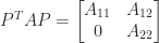
where $A_{11}$ and $A_{22}$ are square, nonempty submatrices; it is irreducible if it is not reducible. Examples of reducible matrices are triangular matrices and matrices with a zero row or column. A positive matrix is trivially irreducible.

Theorem 2. (Perron–Frobenius) If $A\in\mathbb{R}^{n\times n}$ is nonnegative and irreducible then

$\rho(A)$ is an eigenvalue of $A$ ,

$\rho(A)>0$ ,

there is a positive eigenvector $x$ such that $Ax = \rho(A) x$ ,

$\rho(A)$ is a simple eigenvalue.

Theorem 3. (Perron) If $A\in\mathbb{R}^{n\times n}$ is positive then Theorem 2 holds and, in addition, $|\lambda| < \rho(A)$ for any eigenvalue $\lambda$ with $\lambda \ne \rho(A)$ .

For nonnegative, irreducible $A$ , the eigenvalue $\rho(A)$ is called the Perron root of $A$ and the corresponding positive eigenvector $x$ , normalized so that $\|x\|_1 = 1$ , is called the Perron vector.

It is a good exercise to apply the theorems to all binary $2\times 2$ matrices. Here are some interesting cases.

$A = \bigl[\begin{smallmatrix}0 & 1 \\ 0 & 0 \end{smallmatrix}\bigr]$ : Theorem 1 says that $\rho(A) = 0$ is an eigenvalue and and that it has a nonnegative eigenvector. Indeed $[1~0]^T$ is an eigenvector. Note that $A$ is reducible and $0$ is a repeated eigenvalue.
$A = \bigl[\begin{smallmatrix}0 & 1 \\ 1 & 0 \end{smallmatrix}\bigr]$ : $A$ is irreducible and Theorem 2 says that $\rho(A)$ is a simple eigenvalue with positive eigenvector. Indeed the eigenvalues are $\pm 1$ and $[1~1]^T/2$ is the Perron vector for the Perron root $1$ . This matrix has two eigenvalues of maximal modulus.
$A = \bigl[\begin{smallmatrix}1 & 1 \\ 1 & 1 \end{smallmatrix}\bigr]$ : Theorem 3 says that $\rho(A) = 2$ is an eigenvalue with positive eigenvector and that the other eigenvalue has modulus less than $2$ . Indeed the eigenvalues are the Perron root $2$ , with Perron vector $[1~1]^T/2$ , and $0$ .

For another example, consider the irreducible matrix

$\notag B = \begin{bmatrix} 0 & 0 & 1\\ 1 & 0 & 0\\ 0 & 1 & 0 \end{bmatrix}, \quad \Lambda(B) = \bigl\{ 1, \textstyle\frac{1}{2}( -1 \pm \sqrt{3}\mskip1mu\mathrm{i} ) \bigr\}.$

Note that $B$ is a companion matrix and a permutation matrix. Theorem 2 correctly tells us that $\rho(A) = 1$ is an eigenvalue of $A$ , and that it has a corresponding positive eigenvector, the Perron vector $[1~1~1]^T/3$ . Two of the eigenvalues are complex, however, and all three eigenvalues have modulus 1, as they must because $B$ is orthogonal.

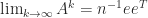
A stochastic matrix is a nonnegative matrix whose row sums are all equal to $1$ . A stochastic matrix satisfies $Ae = e$ , where $e = [1,1,\dots,1]^T$ , which means that $A$ has an eigenvalue $1$ , and so $\rho(A) \ge 1$ . Since $\rho(A) \le \|A\|$ for any norm, by taking the $\infty$ -norm we conclude that $\rho(A) = 1$ . For a stochastic matrix, Theorem 1 does not give any further information. If $A$ is irreducible then Theorem 2 tells us that $\rho(A)$ is a simple eigenvalue, and if $A$ is positive Theorem 3 tells us that every other eigenvalue has modulus less than $\rho(A)$ .

The next result is easily proved using Theorem 3 together with the Jordan canonical form. It shows that the powers of a positive matrix behave like multiples of a rank-1 matrix.

Theorem 4. If $A\in\mathbb{R}^{n\times n}$ is positive, $x$ is the Perron vector of $A$ , and $y$ is the Perron vector of $A^T$ then

$\notag \displaystyle\lim_{k\to\infty} \left( \displaystyle\frac{A}{\rho(A)} \right)^k = \displaystyle\frac{xy^T}{y^Tx}.$

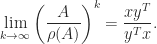
Note that $y$ in the theorem is a left eigenvector of $A$ corresponding to $\rho(A)$ , that is, $y^TA = \rho(A)y^T$ (since $\rho(A^T) = \rho(A)$ ).

If $A$ is stochastic and positive then Theorem 4 is applicable and $x = n^{-1}e$ . If $A$ also has unit column sums, so that it is doubly stochastic, then $y = n^{-1}e$ and Theorem 4 says that $\lim_{k\to\infty}A^k = n^{-1}ee^T$ . We illustrate this result in MATLAB using a scaled magic square matrix.

>> n = 4; M = magic(n), A = M/sum(M(1,:)) % Doubly stochastic matrix.
A =
    16     2     3    13
     5    11    10     8
     9     7     6    12
     4    14    15     1
A =
   4.7059e-01   5.8824e-02   8.8235e-02   3.8235e-01
   1.4706e-01   3.2353e-01   2.9412e-01   2.3529e-01
   2.6471e-01   2.0588e-01   1.7647e-01   3.5294e-01
   1.1765e-01   4.1176e-01   4.4118e-01   2.9412e-02

>> for k = 8:8:32, fprintf('%11.2e',norm(A^k-ones(n)/n,1)), end, disp(' ')
   3.21e-05   7.37e-10   1.71e-14   8.05e-16

References

This is a minimal set of references, which contain further useful references within.

Roger A. Horn and Charles R. Johnson, Matrix Analysis, second edition, Cambridge University Press, 2013. Chapter 8. My review of the second edition.
Carl D. Meyer, Matrix Analysis and Applied Linear Algebra, Society for Industrial and Applied Mathematics, Philadelphia, PA, USA, 2000. Chapter 8.
Helene Shapiro, Linear Algebra and Matrices. Topics for a Second Course, American Mathematical Society, Providence, RI, USA, 2015. Chapter 17.

This article is part of the “What Is” series, available from https://nhigham.com/category/what-is and in PDF form from the GitHub repository https://github.com/higham/what-is.

5 thoughts on “What Is the Perron–Frobenius Theorem?”

Hi, and thanks for the nice post.
In the $2 \times 2$ example: “…eigenvector and that the other eigenvalue has modulus less than 1” I think you meant to write “less than 2”.

Nick Higham says:

July 19, 2021 at 1:43 pm

Thanks – corrected.

Reply

I am hoping PFT will help prove a seemingly simple thing:

For square non negative Q with spectral radius < 1, (I hope that)

(I + Q)^{-1}Q is also non negative.

Any hints or thoughts?

Nick Higham says:

May 31, 2023 at 2:32 pm

It’s false. Here is a counterexample in MATLAB:

>> rng(6); n=2; A = rand(n)/(1.1*max(abs(eig(A)))); (eye(n)+A)\A
ans =
2.3058e-01 2.3561e-01
9.5246e-02 -1.3619e-02

With a change of sign, (I-Q)^{-1}Q is nonnegative, as can be seen
from a Neumann expansion of the inverse.

Reply
1. Ralph Kelsey says:
  
  May 31, 2023 at 3:11 pm
  
  thanks. now I see why I couldn’t prove it. I will have to think if I really need it.
  
  Reply

References

Share this:

Related

5 thoughts on “What Is the Perron–Frobenius Theorem?”

Leave a Reply Cancel reply