Mathematical Word Processing: Historical Snippets

Matthew G. Kirschenbaum’s recent book Track Changes: A Literary History of Word Processing contains a lot of interesting detail about the early days of word processing, covering the period 1964 to 1984. Most of the book concerns non-scientific writing, though $\TeX$ gets a brief mention.

Inspired by the book, I thought it might be useful to collect some information on early mathematical wordprocessing. Little information of this kind seems to be available online.

It is first worth noting that before the advent of word processors papers were typed on a typewriter and mathematical symbols were typically filled in by hand, as in this example from A Study of the Matrix Exponential (1975) by Charlie Van Loan:

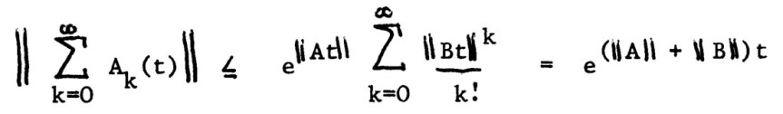
Some institutions had the luxury of IBM Selectric typewriters, which had a “golf ball” that could be changed in order to type special characters. (See this page for informative videos about the Selectric.) Here is an example of output from the Selectric, taken from my MSc thesis: This illustrates some characteristic weaknesses of typewriter output: superscripts, subscripts, and operators are of the same size as the main symbols and spacing between characters is fixed (as in the vertical bars making up the norm signs here).

In 1980s at the Department of Mathematics at the University of Manchester the word processor Vuwriter was used. It was produced by a spin-off company Vuman Computer Systems, which took its name from “Victoria University of Manchester”, the university’s full name. Vuwriter ran on the Apricot PC, produced by the British company Apricot computers. At least one of my first papers was typed on Vuwriter by the office staff and I still have the original 1984 technical report Computing the Polar Decomposition—with Applications, which I have scanned and is available here. A typical equation from the report is this one:

The article

Peter Dolton, Comparing Scientific Word Processor Packages: $T^3$ and Vuwriter, The Economic Journal 100, 311-315, 1990

reviews a version of Vuwriter that ran under MS DOS on IBM PC compatibles. Another review is

D. L. Mealand, Word Processing in Greek using Vuwriter Arts: A Test case for Foreign Language Word Processing, Literary and Linguistic Computing 2, 30-33, 1987

which describes a version of the program for use with foreign languages.

The Department of Mathematics at UMIST (which merged with the University of Manchester in 2004) used an MSDOS word processor called ChiWriter.

In the same period I also prepared manuscripts on my own microcomputers: first on a Commodore 64 and then on a Commodore 128 (essentially a Commodore 64 with a screen 80 characters wide rather than 40 characters wide), using a wordprocessor called Vizawrite. For output I used an Epson FX-80 dot matrix printer, and later an Epson LQ 850 (which produced high resolution output thanks to its 24 pin print head, as opposed to the 9 pin print head of the FX-80). Vizawrite was able to take advantage of the Epson printers’ ability to produce subscripts and superscripts, Greek characters, and mathematical symbols. An earlier post links to a scan of my 1985 article Matrix Computations in Basic on a Microcomputer produced in Vizawrite.

In the 1980s some colleagues wrote papers on a Mac. An example (preserved at the Cornell eCommons digital repository) is A Storage Efficient WY Representation for Products of Householder Transformations (1987) by Charlie Van Loan. I think that report was prepared in Mac Write. Here is a sample equation:

Also in the 1980s I built a database of papers that I had read, and wrote a program that could extract the items that I wanted to cite, format them, and print a sorted list. This was a big time-saver for producing reference lists, especially for my PhD thesis. The database was originally held in Superbase for the Commodore C128, with the program written in Superbase’s own language, and was later transferred to PC-File running on an IBM PC-clone with the program converted to GW-Basic. I was essentially building my own much simpler version of BibTeX, which did not exist when I started the database.

I am aware of two good sources of information about technical word processors for the IBM PC. The first is the article

P. K. Wong, Choices for Mathematical Wordprocessing Software, SIAM News 17(6), pp. 8-9, 1984

This article notes that

“There are over 120 wordprocessing programs for the IBM PC alone and the machine is not yet three years old! Of this large number, however, less than half a dozen can claim scientific wordprocessing capabilities, and these have only been available within the past six to nine months.”

The other source is two articles published in the Notices of the American Mathematical Society in the 1980s.

PC Technical Group of IBM PC Users Group of the Boston Computer Society, Technical Wordprocessors for the IBM PC and Compatibles, Notices Amer. Math. Soc. 33, 8-37, 1986

PC Technical Group of IBM PC Users Group of the Boston Computer Society, Technical Wordprocessors for the IBM PC and Compatibles, Part IIB: Reviews, Notices Amer. Math. Soc. 34, 462-491, 1987

These two articles do not appear to be available online. The first of them includes a set of benchmarks, consisting of extracts from technical journals and books, which were used to test the abilities of the packages. The authors make the interesting comment that

“Microsoft chose not to answer our review request for Word, and based on discussion with Word owners, Word is not set up for equations.”

Finally, Roger Horn told me that his book Topics in Matrix Analysis (CUP, 1991), co-authored with Charlie Johnson, was produced from the camera-ready output of the $T^3$ wordprocessing system (reviewed in this 1988 article and in the SIAM News article above). $T^3$ was chosen because $\TeX$ was not available on PCs when work on the the book began. It must have been a huge effort to produce this 607-page book in this way!

If you have any information to add, please put it in the “Leave a Reply” box below.

Acknowledgement: thanks to Christopher Baker and David Silvester for comments on a draft of this post.

Implicit Expansion: A Powerful New Feature of MATLAB R2016b

The latest release of MATLAB, R2016b, contains a feature called implicit expansion, which is an extension of the scalar expansion that has been part of MATLAB for many years. Scalar expansion is illustrated by

>> A = spiral(2), B = A - 1
A =
     1     2
     4     3
B =
     0     1
     3     2

Here, MATLAB subtracts 1 from every element of A, which is equivalent to expanding the scalar 1 into a matrix of ones then subtracting that matrix from A.

Implicit expansion takes this idea further by expanding vectors:

>> A = ones(2), B = A + [1 5]
A =
     1     1
     1     1
B =
     2     6
     2     6

Here, the result is the same as if the row vector was replicated along the first dimension to produce the matrix [1 5; 1 5] then that matrix was added to ones(2). In the next example a column vector is added and the replication is across the columns:

>> A = ones(2) + [1 5]'
A =
     2     2
     6     6

Implicit expansion also works with multidimensional arrays, though we will focus here on matrices and vectors.

So MATLAB now treats “matrix plus vector” as a legal operation. This is a controversial change, as it means that MATLAB now allows computations that are undefined in linear algebra.

Why have MathWorks made this change? A clue is in the R2016b Release Notes, which say

For example, you can calculate the mean of each column in a matrix A, then subtract the vector of mean values from each column with A - mean(A).

This suggests that the motivation is, at least partly, to simplify the coding of manipulations that are common in data science.

Implicit expansion can also be achieved with the function bsxfun that was introduced in release R2007a, though I suspect that few MATLAB users have heard of this function:

>> A = [1 4; 3 2], bsxfun(@minus,A,mean(A))
A =
     1     4
     3     2
ans =
    -1     1
     1    -1

>> A - mean(A)
ans =
    -1     1
     1    -1

Prior to the introduction of bsxfun, the repmat function could be used to explicitly carry out the expansion, though less efficiently and less elegantly:

>> A - repmat(mean(A),size(A,1),1)
ans =
    -1     1
     1    -1

An application where the new functionality is particularly attractive is multiplication by a diagonal matrix.

>> format short e
>> A = ones(3); d = [1 1e-4 1e-8];
>> A.*d  %  A*diag(d)
ans =
   1.0000e+00   1.0000e-04   1.0000e-08
   1.0000e+00   1.0000e-04   1.0000e-08
   1.0000e+00   1.0000e-04   1.0000e-08
>> A.*d' % diag(d)*A
ans =
   1.0000e+00   1.0000e+00   1.0000e+00
   1.0000e-04   1.0000e-04   1.0000e-04
   1.0000e-08   1.0000e-08   1.0000e-08

The .* expressions are faster than forming and multiplying by diag(d) (as is the syntax bsxfun(@times,A,d)). We can even multiply with the inverse of diag(d) with

>> A./d
ans =
           1       10000   100000000
           1       10000   100000000
           1       10000   100000000

It is now possible to add a column vector to a row vector, or to subtract them:

>> d = (1:3)'; d - d'
ans =
     0    -1    -2
     1     0    -1
     2     1     0

This usage allows very short expressions for forming the Hilbert matrix and Cauchy matrices (look at the source code for hilb.m with type hilb or edit hilb).

The max and min functions support implicit expansion, so an elegant way to form the matrix $A$ with $(i,j)$ element $\min(i,j)$ is with

d = (1:n); A = min(d,d');

and this is precisely what gallery('minij',n) now does.

Another function that can benefit from implicit expansion is vander, which forms a Vandermonde matrix. Currently the function forms the matrix in three lines, with calls to repmat and cumprod. Instead we can do it as follows, in a formula that is closer to the mathematical definition and hence easier to check.

A = (v(:) .^ (n-1:-1:0)')';  % Equivalent to A = vander(v)

The latter code is, however, slower than the current vander for large dimensions, presumably because exponentiating each element independently is slower than using repeated multiplication.

An obvious objection to implicit expansion is that it could cause havoc in linear algebra courses, where students will be able to carry out operations that the instructor and textbook have said are not allowed. Moreover, it will allow programs with certain mistyped expressions to run that would previously have generated an error, making debugging more difficult.

I can see several responses to this objection. First, MATLAB was already inconsistent with linear algebra in its scalar expansion. When a mathematician writes (with a common abuse of notation) $A - \sigma$ , with a scalar $\sigma$ , he or she usually means $A - \sigma I$ and not $A - \sigma E$ with $E$ the matrix of ones.

Second, I have been using the prerelease version of R2016b for a few months, while working on the third edition of MATLAB Guide, and have not encountered any problems caused by implicit expansion—either with existing codes or with new code that I have written.

A third point in favour of implicit expansion is that it is particularly compelling with elementwise operations (those beginning with a dot), as the multiplication by a diagonal matrix above illustrates, and since such operations are not a part of linear algebra confusion is less likely.

Finally, it is worth noting that implicit expansion fits into the MATLAB philosophy of “useful defaults” or “doing the right thing”, whereby MATLAB makes sensible choices when a user’s request is arguably invalid or not fully specified. This is present in the many functions that have optional arguments. But it can also be seen in examples such as

% No figure is open and no parallel pool is running.
>> close         % Close figure.
>> delete(gcp)   % Shut down parallel pool.

where no error is generated even though there is no figure to close or parallel pool to shut down.

I suspect that people’s reactions to implicit expansion will be polarized: they will either be horrified or will regard it as natural and useful. Now that I have had time to get used to the concept—and especially now that I have seen the benefits both for clarity of code (the minij matrix) and for speed (multiplication by a diagonal matrix)—I like it. It will be interesting to see the community’s reaction.

Second Edition (2016) of Learning LaTeX by David Griffiths and Des Higham

What is the best way to learn $\LaTeX$ ? Many free online resources are available, including “getting started” guides, FAQs, references, Wikis, and so on. But in my view you can’t beat using a (physical) book. A book can be read anywhere. You can write notes in it, stick page markers on it, and quickly browse it or look something up in the index.

The first edition of Learning $\LaTeX$ (1997) is a popular introduction to $\LaTeX$ characterized by its brevity, its approach of teaching by example, and its humour. (Full disclosure: the second author is my brother.)

The second edition of the book is 25 percent longer than the first and has several key additions. The amsmath package, particularly of interest for its environments for typesetting multiline equations, is now described. I often struggle to remember the differences between align, alignat, gather, and multline, but three pages of concise examples explain these environments very clearly.

The book now reflects the modern PDF workflow, based on pdflatex as the $\TeX$ engine. If you are still generating dvi files you should consider making the switch!

Other features new to this edition are a section on making bibliographies with Bib $\TeX$ and appendices on making slides with Beamer and posters with the a0poster class, both illustrated with complete sample documents.

Importantly for a book to be used for reference, there is an excellent 10.5-page index which, at about 10% of the length of the book, is unusually thorough (see the discussion on index length in my A Call for Better Indexes).

The 1997 first edition was reviewed in TUGboat (the journal of the TeX Users Group) in 2013 by Boris Veytsman, who had only just become aware of the book. He says

When Karl Berry and I discussed the current situation with $\LaTeX$ books for beginners, he mentioned the old text by Grffiths and Higham as an example of the one made “right”…

This is indeed an incredibly good introduction to $\LaTeX$ . Even today, when many good books are available for beginners, this one stands out.

No doubt Berry and Veytsman would be even more impressed by the improved and expanded second edition.

Given that I regard myself as an advanced $\LaTeX$ user I was surprised to learn something I didn’t know from the book, namely that in an \includegraphics command it is not necessary to specify the extension of the file being included. If you write \includegraphics{myfig} then pdflatex will search for myfig.png, myfig.pdf, myfig.jpg, and myfig.eps, in that order. If you specify

\DeclareGraphicsExtensions{.pdf,.png,.jpg}

in the preamble, $\LaTeX$ will search for the given extensions in the specified order. I usually save my figures in PDF form, but sometimes a MATLAB figure saved as a jpeg file is much smaller.

This major update of the first edition is beautifully typeset, printed on high quality, bright white paper, and weighs just 280g. It is an excellent guide for those new to $\LaTeX$ and a useful reference for experienced users.

Share this:

Share this:

Share this: