A symmetric indefinite matrix 


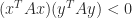
A neat way to express the indefinitess is that there exist vectors 
A symmetric indefinite matrix has both positive and negative eigenvalues and in some sense is a typical symmetric matrix. For example, a random symmetric matrix is usually indefinite:
>> rng(3); B = rand(4); A = B + B'; eig(A)'
ans =
  -8.9486e-01  -6.8664e-02   1.1795e+00   3.9197e+00
In general it is difficult to tell if a symmetric matrix is indefinite or definite, but there is one easy-to-spot sufficient condition for indefinitess: if the matrix has a zero diagonal element that has a nonzero element in its row then it is indefinite. Indeed if 


An example of a symmetric indefinite matrix is a saddle point matrix, which has the block 

where 


which has eigenvalues 


>> A = full(gallery('tridiag',5,1,0,1)), eig(sym(A))'
A =
     0     1     0     0     0
     1     0     1     0     0
     0     1     0     1     0
     0     0     1     0     1
     0     0     0     1     0
ans =
[-1, 0, 1, 3^(1/2), -3^(1/2)]
How can we exploit symmetry in solving a linear system 


The way round this is to allow 


MATLAB implements ldl function. Here is an example using Anymatrix:
>> A = anymatrix('core/blockhouse',4), [L,D,P] = ldl(A), eigA = eig(A)'
A =
  -4.0000e-01  -8.0000e-01  -2.0000e-01   4.0000e-01
  -8.0000e-01   4.0000e-01  -4.0000e-01  -2.0000e-01
  -2.0000e-01  -4.0000e-01   4.0000e-01  -8.0000e-01
   4.0000e-01  -2.0000e-01  -8.0000e-01  -4.0000e-01
L =
   1.0000e+00            0            0            0
            0   1.0000e+00            0            0
   5.0000e-01  -8.3267e-17   1.0000e+00            0
  -2.2204e-16  -5.0000e-01            0   1.0000e+00
D =
  -4.0000e-01  -8.0000e-01            0            0
  -8.0000e-01   4.0000e-01            0            0
            0            0   5.0000e-01  -1.0000e+00
            0            0  -1.0000e+00  -5.0000e-01
P =
     1     0     0     0
     0     1     0     0
     0     0     1     0
     0     0     0     1
eigA =
  -1.0000e+00  -1.0000e+00   1.0000e+00   1.0000e+00
Notice the
References
- Cleve Ashcraft, Roger Grimes, and John Lewis, Accurate Symmetric Indefinite Linear Equation Solvers, SIAM J. Matrix Anal. Appl. 20, 513–561, 1998.
- Nicholas J. Higham and Mantas Mikaitis, Anymatrix: An Extendable MATLAB Matrix Collection, Numer. Algorithms, 90:3, 1175–1196, 2021.
Related Blog Posts
- What Is a Modified Cholesky Factorization? (2020)
- What Is a Symmetric Positive Definite Matrix? (2020)
This article is part of the “What Is” series, available from https://nhigham.com/category/what-is and in PDF form from the GitHub repository https://github.com/higham/what-is.
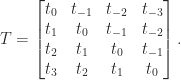
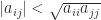
 is a Toeplitz matrix if
  for
for  parameters
  . A Toeplitz matrix has constant diagonals. For
  :
:
 .
. can be solved in less than the
  flops that would be required by LU factorization. Indeed methods are available that require only
  flops; see Golub and Van Loan (2013) for details.
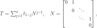
 is upper bidiagonal with a superdiagonal of ones and
  . It follows that the product of two upper triangular Toeplitz matrices is again upper triangular Toeplitz, upper triangular Toeplitz matrices commute, and
  is also an upper triangular Toeplitz matrix (assuming
  is nonzero, so that
  is nonsingular).
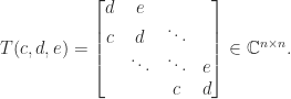
 are
are
 equations in
  , where
  is the matrix inverse. What is not always emphasized is that there are very few circumstances in which one should compute
  ) system
  by computing
  , but rather would carry out a division
  . In the
 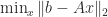 , where
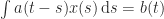
  matrix with
  , satisfies the normal equations
  . It is therefore natural to form the symmetric positive definite matrix
  and solve the normal equations by Cholesky factorization. While fast, this method is numerically unstable when
 is the unit roundoff of the floating point arithmetic, then
 , in floating-point arithmetic
  rounds to
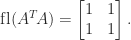
 has been lost.
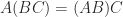 , and in general the cost of the evaluation of a product depends on where one puts the parentheses. One order may be much superior to others, so one should not simply evaluate the product in a fixed left-right or right-left order. For example, if
  are
are  can be evaluated as
 : a vector outer product followed by a matrix–vector product, costing
  : a vector scalar product followed by a vector scaling, costing just
  operations.
 in order to minimize the operation count is a
  ,
, for all
  ,
, factor is returned in the first argument, and it can be used to compute a direction of negative curvature (as needed in optimization), for example.
 that exploit the block structure and possible sparsity in
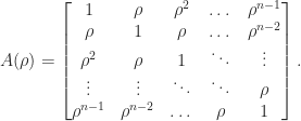
  . A second example is a circulant matrix
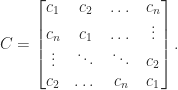
 in
in  operations, rather than the
  indicates a matrix that is nearly singular. However, the size of
 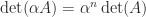 we can achieve any value for the determinant by multiplying by a scalar
  , yet
, yet  is no more or less nearly singular than
  .
.
 , yet
, yet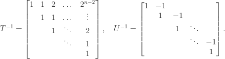
 element of
  then the matrix becomes singular! By contrast,
  is always very well conditioned. The determinant cannot distinguish between the ill-conditioned
  for all
  , where the
  are the eigenvalue of
  , it follows that the matrix condition number
  is bounded below by the ratio of largest to smallest eigenvalue in absolute value, that is,

 is a singular value decomposition (SVD), with
  orthogonal and
  ,
,  . If
. If  and
and  are the same, but in general the eigenvalues
  can be very different.