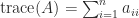
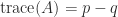
The trace of an 

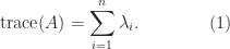
A key fact is that the trace is also the sum of the eigenvalues. The proof is by considering the characteristic polynomial 


and so 


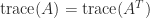
A consequence of (1) is that any transformation that preserves the eigenvalues preserves the trace. Therefore the trace is unchanged under similarity transformations: 

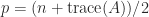
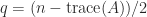
An an example of how the trace can be useful, suppose 


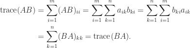
Another important property is that for an 


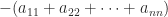
(despite the fact that 
This simple fact can have non-obvious consequences. For example, consider the equation 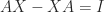

The relation (2) gives 


So we can cyclically permute terms in a matrix product without changing the trace.
As an example of the use of (2) and (3), if 


The trace is useful in calculations with the Frobenius norm of an
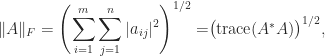
where 

where 

If a matrix is not explicitly known but we can compute matrix–vector products with it then the trace can be estimated by
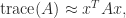
where the vector 

since 


References
- Haim Avron and Sivan Toledo, Randomized Algorithms for Estimating the Trace of an Implicit Symmetric Positive Semi-definite Matrix, J. ACM 58, 8:1-8:34, 2011.
Related Blog Posts
- What Is a Matrix Norm? (2021)
- What Is an Eigenvalue? (2022)
This article is part of the “What Is” series, available from https://nhigham.com/category/what-is and in PDF form from the GitHub repository https://github.com/higham/what-is.
 is diagonalizable if there exists a nonsingular matrix
  such that
  is diagonal. In other words, a diagonalizable matrix is one that is similar to a diagonal matrix.
 is equivalent to
  with
with  ,
,  , where
 ![X = [x_1,x_2,\dots, x_n]](https://s0.wp.com/latex.php?latex=X+%3D+%5Bx_1%2Cx_2%2C%5Cdots%2C+x_n%5D&bg=ffffff&fg=222222&s=0&c=20201002) . Hence
. Hence  ). A matrix with distinct eigenvalues is also diagonalizable.
 has distinct eigenvalues then it is diagonalizable.
 with corresponding eigenvectors
  . Suppose that
 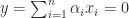 for some
  . Then
 since
since  for
for  and
and  . Premultiplying
  by
by 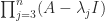 shows, in the same way, that
  . Continuing in this way we find that
  . Therefore the
  are linearly independent and hence
  -times repeated eigenvalue has
 ![\bigl[\begin{smallmatrix} 0 & 1 \\ 0 & 0 \end{smallmatrix}\bigr]](https://s0.wp.com/latex.php?latex=%5Cbigl%5B%5Cbegin%7Bsmallmatrix%7D+0+%26+1+%5C%5C+0+%26+0+%5Cend%7Bsmallmatrix%7D%5Cbigr%5D&bg=ffffff&fg=222222&s=0&c=20201002) . This matrix is a
. This matrix is a  Jordan block with the eigenvalue
  .
. , that is, any matrix in
  diagonalizable, where
  are nonzero? There are
  zero eigenvalues with eigenvectors any set of linearly independent vectors orthogonal to
  then
then  is the remaining eigenvalue, with eigenvector
  then all the eigenvalues of
 ![x = \bigl[{1 \atop 0} \bigr]](https://s0.wp.com/latex.php?latex=x+%3D+%5Cbigl%5B%7B1+%5Catop+0%7D+%5Cbigr%5D&bg=ffffff&fg=222222&s=0&c=20201002) and
and ![y = \bigl[{0 \atop 1} \bigr]](https://s0.wp.com/latex.php?latex=y+%3D+%5Cbigl%5B%7B0+%5Catop+1%7D+%5Cbigr%5D&bg=ffffff&fg=222222&s=0&c=20201002) , so
, so 