In many situations we need to evaluate the derivative of a function but we do not have an explicit formula for the derivative. The complex step approximation approximates the derivative (and the function value itself) from a single function evaluation. The catch is that it involves complex arithmetic.
For an analytic function  we have the Taylor expansion

where  is the imaginary unit. Assume that maps the real line to the real line and that
  and
and  are real. Then equating real and imaginary parts in
  gives
gives  and
and  . This means that for small , the approximations
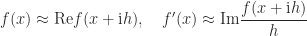
both have error  . So a single evaluation of at a complex argument gives, for small , a good approximation to
  , as well as a good approximation to
  if we need it.
The usual way to approximate derivatives is with finite differences, for example by the forward difference approximation

This approximation has error  so it is less accurate than the complex step approximation for a given , but more importantly it is prone to numerical cancellation. For small ,
  and agree to many significant digits and so in floating-point arithmetic the difference approximation suffers a loss of significant digits. Consequently, as decreases the error in the computed approximation eventually starts to increase. As numerical analysis textbooks explain, the optimal choice of that balances truncation error and rounding errors is approximately
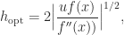
where  is the unit roundoff. The optimal error is therefore of order
  .
.
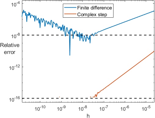
A simple example illustrate these ideas. For the function  with
with  , we plot in the figure below the relative error for the finite difference, in blue, and the relative error for the complex step approximation, in orange, for ranging from about
  to
to  . The dotted lines show and . The computations are in double precision (
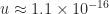 ). The finite difference error decreases with until it reaches about
  ; thereafter the error grows, giving the characteristic V-shaped error curve. The complex step error decreases steadily until it is of order for
  , and for each it is about the square of the finite difference error, as expected from the theory.
Remarkably, one can take extremely small in the complex step approximation (e.g.,  ) without any ill effects from roundoff.
The complex step approximation carries out a form of approximate automatic differentiation, with the variable functioning like a symbolic variable that propagates through the computations in the imaginary parts.
The complex step approximation applies to gradient vectors and it can be extended to matrix functions. If is analytic and maps real  matrices to real matrices and
  and
and  are real then (Al-Mohy and Higham, 2010)

where  is the Fréchet derivative of at in the direction . It is important to note that the method used to evaluate must not itself use complex arithmetic (as methods based on the Schur decomposition do); if it does, then the interaction of those complex terms with the much smaller
  term can lead to damaging subtractive cancellation.
The complex step approximation has also been extended to higher derivatives by using “different imaginary units” in different components (Lantoine et al., 2012).
Here are some applications where the complex step approximation has been used.
- Sensitivity analysis in engineering applications (Giles et al., 2003).
- Approximating gradients in deep learning (Goodfellow et al., 2016).
- Approximating the exponential of an operator in option pricing (Ackerer and Filipović, 2019).
Software has been developed for automatically carrying out the complex step method—for example, by Shampine (2007).
The complex step approximation has been rediscovered many times. The earliest published appearance that we are aware of is in a paper by Squire and Trapp (1998), who acknowledge earlier work of Lyness and Moler on the use of complex variables to approximate derivatives.
References
This is a minimal set of references, which contain further useful references within.
- Awad H. Al-Mohy and Nicholas J. Higham, The Complex Step Approximation to the Fréchet Derivative of a Matrix Function, Numer. Algorithms 53, 133–148, 2010.
- Damien Ackerer and Damir Filipović, Option Pricing with Orthogonal Polynomial Expansions, Mathematical Finance 30, 47–84, 2019.
- Michael B. Giles, Mihai C. Duta, Jens-Dominik Möuller, and Niles A. Pierce, Algorithm Developments for Discrete Adjoint Methods, AIAA Journal 4(2), 198–205, 2003.
- Ian Goodfellow, Yoshua Bengio, and Aaron Courville, Deep Learning, MIT Press, 2016. Page 434.
- Gregory Lantoine, Ryan P. Russell P., and Thierry Dargent, Using Multicomplex Variables for Automatic Computation of High-Order Derivatives, ACM Trans. Math. Software 38, 16:1–16:21, 2012.
- L. F. Shampine, Accurate Numerical Derivatives in MATLAB, ACM Trans. Math. Software 33,26:1–26:17, 2007.
- W. Squire and G. E. Trapp (1998), Using Complex Variables to Estimate Derivatives of Real Functions, SIAM Rev., 40(1), 110–112.


![\notag Q = \begin{array}[b]{@{\mskip35mu}c@{\mskip-20mu}c@{\mskip-10mu}c@{}} \scriptstyle p & \scriptstyle p & \\ \multicolumn{2}{c}{ \left[\begin{array}{c@{~}c@{~}} Q_{11}& Q_{12} \\ Q_{21}& Q_{22} \\ \end{array}\right]} & \mskip-12mu\ \begin{array}{c} \scriptstyle p \\ \scriptstyle p \end{array} \end{array}.](https://s0.wp.com/latex.php?latex=%5Cnotag++++Q+%3D++++%5Cbegin%7Barray%7D%5Bb%5D%7B%40%7B%5Cmskip35mu%7Dc%40%7B%5Cmskip-20mu%7Dc%40%7B%5Cmskip-10mu%7Dc%40%7B%7D%7D++++%5Cscriptstyle+p+%26++++%5Cscriptstyle+p+%26++++%5C%5C++++%5Cmulticolumn%7B2%7D%7Bc%7D%7B++++++++%5Cleft%5B%5Cbegin%7Barray%7D%7Bc%40%7B%7E%7Dc%40%7B%7E%7D%7D++++++++++++++++++Q_%7B11%7D%26+Q_%7B12%7D+%5C%5C++++++++++++++++++Q_%7B21%7D%26+Q_%7B22%7D+%5C%5C++++++++++++++%5Cend%7Barray%7D%5Cright%5D%7D++++%26+%5Cmskip-12mu%5C++++++++++%5Cbegin%7Barray%7D%7Bc%7D++++++++++++++%5Cscriptstyle+p+%5C%5C++++++++++++++%5Cscriptstyle+p++++++++++++++%5Cend%7Barray%7D++++%5Cend%7Barray%7D.+&bg=ffffff&fg=222222&s=0&c=20201002)
![\notag \begin{bmatrix} U_1^T & 0\\ 0 & U_2^T \end{bmatrix} \begin{bmatrix} Q_{11} & Q_{12}\\ Q_{21} & Q_{22} \end{bmatrix} \begin{bmatrix} V_1 & 0\\ 0 & V_2 \end{bmatrix} = \begin{array}[b]{@{\mskip36mu}c@{\mskip-13mu}c@{\mskip-10mu}c@{}} \scriptstyle p & \scriptstyle p & \\ \multicolumn{2}{c}{ \left[\begin{array}{@{\mskip3mu}rr@{~}} C & S \\ -S & C \end{array}\right]} & \mskip-12mu\ \begin{array}{c} \scriptstyle p \\ \scriptstyle p \end{array} \end{array},](https://s0.wp.com/latex.php?latex=%5Cnotag++++%5Cbegin%7Bbmatrix%7D++U_1%5ET+%26+0%5C%5C++++++++++++++++++++++++++0+++%26+U_2%5ET++++%5Cend%7Bbmatrix%7D++++%5Cbegin%7Bbmatrix%7D++Q_%7B11%7D+%26+Q_%7B12%7D%5C%5C++++++++++++++++++++++++++Q_%7B21%7D+%26+Q_%7B22%7D++++%5Cend%7Bbmatrix%7D++++%5Cbegin%7Bbmatrix%7D++V_1+%26+0%5C%5C++++++++++++++++++++++++++0+++%26+V_2++++%5Cend%7Bbmatrix%7D++++%3D++++%5Cbegin%7Barray%7D%5Bb%5D%7B%40%7B%5Cmskip36mu%7Dc%40%7B%5Cmskip-13mu%7Dc%40%7B%5Cmskip-10mu%7Dc%40%7B%7D%7D++++%5Cscriptstyle+p+%26++++%5Cscriptstyle+p+%26++++%5C%5C++++%5Cmulticolumn%7B2%7D%7Bc%7D%7B++++++++%5Cleft%5B%5Cbegin%7Barray%7D%7B%40%7B%5Cmskip3mu%7Drr%40%7B%7E%7D%7D++++++++++++++++++C+%26++++S+++++++++%5C%5C+++++++++++++++++-S+%26++++C++++++++++++++%5Cend%7Barray%7D%5Cright%5D%7D++++%26+%5Cmskip-12mu%5C++++++++++%5Cbegin%7Barray%7D%7Bc%7D++++++++++++++%5Cscriptstyle+p+%5C%5C++++++++++++++%5Cscriptstyle+p++++++++++++++%5Cend%7Barray%7D++++%5Cend%7Barray%7D%2C+&bg=ffffff&fg=222222&s=0&c=20201002)


![\left[\begin{smallmatrix} c & s \\ -s & c \end{smallmatrix}\right]](https://s0.wp.com/latex.php?latex=%5Cleft%5B%5Cbegin%7Bsmallmatrix%7D+c+%26+s+%5C%5C+-s+%26+c+%5Cend%7Bsmallmatrix%7D%5Cright%5D&bg=ffffff&fg=222222&s=0&c=20201002)


![\notag Q = \begin{array}[b]{@{\mskip33mu}c@{\mskip-16mu}c@{\mskip-10mu}c@{}} \scriptstyle p & \scriptstyle n-p & \\ \multicolumn{2}{c}{ \left[\begin{array}{c@{~}c@{~}} Q_{11}& Q_{12} \\ Q_{21}& Q_{22} \\ \end{array}\right]} & \mskip-12mu\ \begin{array}{c} \scriptstyle p \\ \scriptstyle n-p \end{array} \end{array}, \quad p \le \displaystyle\frac{n}{2}.](https://s0.wp.com/latex.php?latex=%5Cnotag++++Q+%3D++++%5Cbegin%7Barray%7D%5Bb%5D%7B%40%7B%5Cmskip33mu%7Dc%40%7B%5Cmskip-16mu%7Dc%40%7B%5Cmskip-10mu%7Dc%40%7B%7D%7D++++%5Cscriptstyle+p+%26++++%5Cscriptstyle+n-p+%26++++%5C%5C++++%5Cmulticolumn%7B2%7D%7Bc%7D%7B++++++++%5Cleft%5B%5Cbegin%7Barray%7D%7Bc%40%7B%7E%7Dc%40%7B%7E%7D%7D++++++++++++++++++Q_%7B11%7D%26+Q_%7B12%7D+%5C%5C++++++++++++++++++Q_%7B21%7D%26+Q_%7B22%7D+%5C%5C++++++++++++++%5Cend%7Barray%7D%5Cright%5D%7D++++%26+%5Cmskip-12mu%5C++++++++++%5Cbegin%7Barray%7D%7Bc%7D++++++++++++++%5Cscriptstyle+p+%5C%5C++++++++++++++%5Cscriptstyle+n-p++++++++++++++%5Cend%7Barray%7D++++%5Cend%7Barray%7D%2C+%5Cquad+p+%5Cle+%5Cdisplaystyle%5Cfrac%7Bn%7D%7B2%7D.+&bg=ffffff&fg=222222&s=0&c=20201002)
![\notag \begin{bmatrix} U_1^T & 0\\ 0 & U_2^T \end{bmatrix} \begin{bmatrix} Q_{11} & Q_{12}\\ Q_{21} & Q_{22} \end{bmatrix} \begin{bmatrix} V_1 & 0\\ 0 & V_2 \end{bmatrix} = \begin{array}[b]{@{\mskip35mu}c@{\mskip30mu}c@{\mskip-10mu}c@{}c} \scriptstyle p & \scriptstyle p & \scriptstyle n-2p & \\ \multicolumn{3}{c}{ \left[\begin{array}{c@{~}|c@{~}c} C & S & 0 \\ \hline -S & C & 0 \\ 0 & 0 & I_{n-2p} \end{array}\right]} & \mskip-12mu \begin{array}{c} \scriptstyle p \\ \scriptstyle p \\ \scriptstyle n-2p \end{array} \end{array},](https://s0.wp.com/latex.php?latex=%5Cnotag++++%5Cbegin%7Bbmatrix%7D++U_1%5ET+%26+0%5C%5C++++++++++++++++++++++++++0+++%26+U_2%5ET++++%5Cend%7Bbmatrix%7D++++%5Cbegin%7Bbmatrix%7D++Q_%7B11%7D+%26+Q_%7B12%7D%5C%5C++++++++++++++++++++++++++Q_%7B21%7D+%26+Q_%7B22%7D++++%5Cend%7Bbmatrix%7D++++%5Cbegin%7Bbmatrix%7D++V_1+%26+0%5C%5C++++++++++++++++++++++++++0+++%26+V_2++++%5Cend%7Bbmatrix%7D++++%3D++++%5Cbegin%7Barray%7D%5Bb%5D%7B%40%7B%5Cmskip35mu%7Dc%40%7B%5Cmskip30mu%7Dc%40%7B%5Cmskip-10mu%7Dc%40%7B%7Dc%7D++++%5Cscriptstyle+p+%26++++%5Cscriptstyle+p+%26++++%5Cscriptstyle+n-2p+%26++++%5C%5C++++%5Cmulticolumn%7B3%7D%7Bc%7D%7B++++%5Cleft%5B%5Cbegin%7Barray%7D%7Bc%40%7B%7E%7D%7Cc%40%7B%7E%7Dc%7D++++C+%26++++S++++++%26+0+++%5C%5C++++%5Chline+++-S+%26++++C++++++%26+0+++%5C%5C++++0+%26++++0++++++%26+I_%7Bn-2p%7D++++%5Cend%7Barray%7D%5Cright%5D%7D++++%26+%5Cmskip-12mu++++%5Cbegin%7Barray%7D%7Bc%7D++++%5Cscriptstyle+p+%5C%5C++++%5Cscriptstyle+p+%5C%5C++++%5Cscriptstyle+n-2p++++%5Cend%7Barray%7D++++%5Cend%7Barray%7D%2C+&bg=ffffff&fg=222222&s=0&c=20201002)


![\notag \begin{aligned} \left[\begin{array}{rr|rrr} 0.71 & -0.71 & 0 & 0 & 0 \\ -0.71 & -0.71 & 0 & 0 & 0 \\\hline 0 & 0 & 0.17 & 0.61 & -0.78 \\ 0 & 0 & -0.58 & -0.58 & -0.58 \\ 0 & 0 & -0.80 & 0.54 & 0.25 \\ \end{array}\right] \left[\begin{array}{rr|rrr} -0.60 & -0.40 & -0.40 & -0.40 & -0.40 \\ 0.40 & 0.60 & -0.40 & -0.40 & -0.40 \\\hline 0.40 & -0.40 & 0.60 & -0.40 & -0.40 \\ 0.40 & -0.40 & -0.40 & 0.60 & -0.40 \\ 0.40 & -0.40 & -0.40 & -0.40 & 0.60 \\ \end{array}\right] \\ \times \left[\begin{array}{rr|rrr} -0.71 & 0.71 & 0 & 0 & 0 \\ -0.71 & -0.71 & 0 & 0 & 0 \\\hline 0 & 0 & 0.17 & 0.58 & -0.80 \\ 0 & 0 & 0.61 & 0.58 & 0.54 \\ 0 & 0 & -0.78 & 0.58 & 0.25 \\ \end{array}\right] = \left[\begin{array}{rr|rrr} 1.00 & 0 & 0 & 0 & 0 \\ 0 & 0.20 & 0 & 0.98 & 0 \\\hline 0 & 0 & 1.00 & 0 & 0 \\ 0 & -0.98 & 0 & 0.20 & 0 \\ 0 & 0 & 0 & 0 & 1.00 \\ \end{array}\right]. \end{aligned}](https://s0.wp.com/latex.php?latex=%5Cnotag+%5Cbegin%7Baligned%7D+%5Cleft%5B%5Cbegin%7Barray%7D%7Brr%7Crrr%7D++0.71++%26+-0.71++%26++0+++++%26++0+++++%26++0+++++%5C%5C+-0.71++%26+-0.71++%26++0+++++%26++0+++++%26++0+++++%5C%5C%5Chline++0+++++%26++0+++++%26++0.17++%26++0.61++%26+-0.78++%5C%5C++0+++++%26++0+++++%26+-0.58++%26+-0.58++%26+-0.58++%5C%5C++0+++++%26++0+++++%26+-0.80++%26++0.54++%26++0.25++%5C%5C++%5Cend%7Barray%7D%5Cright%5D+%5Cleft%5B%5Cbegin%7Barray%7D%7Brr%7Crrr%7D+-0.60++%26+-0.40++%26+-0.40++%26+-0.40++%26+-0.40++%5C%5C++0.40++%26++0.60++%26+-0.40++%26+-0.40++%26+-0.40++%5C%5C%5Chline++0.40++%26+-0.40++%26++0.60++%26+-0.40++%26+-0.40++%5C%5C++0.40++%26+-0.40++%26+-0.40++%26++0.60++%26+-0.40++%5C%5C++0.40++%26+-0.40++%26+-0.40++%26+-0.40++%26++0.60++%5C%5C+%5Cend%7Barray%7D%5Cright%5D+%5C%5C+%5Ctimes+%5Cleft%5B%5Cbegin%7Barray%7D%7Brr%7Crrr%7D+-0.71++%26++0.71++%26++0+++++%26++0+++++%26++0+++++%5C%5C+-0.71++%26+-0.71++%26++0+++++%26++0+++++%26++0+++++%5C%5C%5Chline++0+++++%26++0+++++%26++0.17++%26++0.58++%26+-0.80++%5C%5C++0+++++%26++0+++++%26++0.61++%26++0.58++%26++0.54++%5C%5C++0+++++%26++0+++++%26+-0.78++%26++0.58++%26++0.25++%5C%5C+%5Cend%7Barray%7D%5Cright%5D+%3D+%5Cleft%5B%5Cbegin%7Barray%7D%7Brr%7Crrr%7D++1.00++%26++0+++++%26++0+++++%26++0+++++%26++0+++++%5C%5C++0+++++%26++0.20++%26++0+++++%26++0.98++%26++0+++++%5C%5C%5Chline++0+++++%26++0+++++%26++1.00++%26++0+++++%26++0+++++%5C%5C++0+++++%26+-0.98++%26++0+++++%26++0.20++%26++0+++++%5C%5C++0+++++%26++0+++++%26++0+++++%26++0+++++%26++1.00++%5C%5C+%5Cend%7Barray%7D%5Cright%5D.+%5Cend%7Baligned%7D+&bg=ffffff&fg=222222&s=0&c=20201002)
: if
then
. When
.
![\notag Q = \begin{array}[b]{@{\mskip-25mu}c@{\mskip-20mu}c@{}} \scriptstyle n \\ \multicolumn{1}{c}{ \left[\begin{array}{@{}c@{}} Q_{1}\\ Q_{2} \end{array}\right]} & \mskip-12mu\ \begin{array}{c} \scriptstyle p \\ \scriptstyle q \end{array} \end{array}, \quad p\ge n, \quad q \ge n.](https://s0.wp.com/latex.php?latex=%5Cnotag++++Q+%3D++++%5Cbegin%7Barray%7D%5Bb%5D%7B%40%7B%5Cmskip-25mu%7Dc%40%7B%5Cmskip-20mu%7Dc%40%7B%7D%7D++++%5Cscriptstyle+n++++%5C%5C++++%5Cmulticolumn%7B1%7D%7Bc%7D%7B++++++++%5Cleft%5B%5Cbegin%7Barray%7D%7B%40%7B%7Dc%40%7B%7D%7D++++++++++++++++++Q_%7B1%7D%5C%5C++++++++++++++++++Q_%7B2%7D++++++++++++++%5Cend%7Barray%7D%5Cright%5D%7D++++%26+%5Cmskip-12mu%5C++++++++++%5Cbegin%7Barray%7D%7Bc%7D++++++++++++++%5Cscriptstyle+p+%5C%5C++++++++++++++%5Cscriptstyle+q++++++++++%5Cend%7Barray%7D++++%5Cend%7Barray%7D%2C+%5Cquad+p%5Cge+n%2C+%5Cquad+q+%5Cge+n.+&bg=ffffff&fg=222222&s=0&c=20201002)
![\notag \begin{bmatrix} U_1^T & 0\\ 0 & U_2^T \end{bmatrix} \begin{bmatrix} Q_{1}\\ Q_{2} \end{bmatrix} V = \begin{array}[b]{@{\mskip-25mu}c@{\mskip-20mu}c@{}} \scriptstyle n \\ \multicolumn{1}{c}{ \left[\begin{array}{c@{~}} C\\ S \end{array}\right]} & \mskip-12mu\ \begin{array}{c} \scriptstyle p \\ \scriptstyle q \end{array} \end{array},](https://s0.wp.com/latex.php?latex=%5Cnotag++++%5Cbegin%7Bbmatrix%7D++U_1%5ET+%26+0%5C%5C++++++++++++++++++++++++++0+++%26+U_2%5ET++++%5Cend%7Bbmatrix%7D++++%5Cbegin%7Bbmatrix%7D++Q_%7B1%7D%5C%5C+++++++++++++++++++++Q_%7B2%7D++++%5Cend%7Bbmatrix%7D++++V++++%3D++++%5Cbegin%7Barray%7D%5Bb%5D%7B%40%7B%5Cmskip-25mu%7Dc%40%7B%5Cmskip-20mu%7Dc%40%7B%7D%7D++++%5Cscriptstyle+n++++%5C%5C++++%5Cmulticolumn%7B1%7D%7Bc%7D%7B++++++++%5Cleft%5B%5Cbegin%7Barray%7D%7Bc%40%7B%7E%7D%7D++++++++++++++++++C%5C%5C++++++++++++++++++S++++++++++++++%5Cend%7Barray%7D%5Cright%5D%7D++++%26+%5Cmskip-12mu%5C++++++++++%5Cbegin%7Barray%7D%7Bc%7D++++++++++++++%5Cscriptstyle+p+%5C%5C++++++++++++++%5Cscriptstyle+q++++++++++%5Cend%7Barray%7D++++%5Cend%7Barray%7D%2C+&bg=ffffff&fg=222222&s=0&c=20201002)


 of a low rank approximation to a matrix (
 and
and  orthogonal,
  -by-
-by- , where
  , where
  is a random
  matrix. The value of
  , where
  is a tolerance that defaults to
  and must not be less than
  , where
  is the machine epsilon (
 for double precision). The algorithm includes a power method iteration that refines the sketch before computing the SVD.
 requested. This is a difficult matrix for
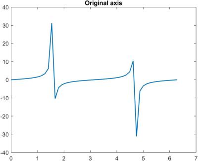


 is a factorization
 and
and  , where
  , and
, and 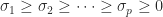 .
.![U =[ u_1,\dots,u_m]](https://s0.wp.com/latex.php?latex=U+%3D%5B+u_1%2C%5Cdots%2Cu_m%5D&bg=ffffff&fg=222222&s=0&c=20201002) and
and ![V = [v_1,\dots, v_n]](https://s0.wp.com/latex.php?latex=V+%3D+%5Bv_1%2C%5Cdots%2C+v_n%5D&bg=ffffff&fg=222222&s=0&c=20201002) . The
. The  are called the singular values of
  and
and  are the left and right singular vectors. We have
  ,
,  . The matrix
  is unique but
 ![\notag \Sigma = \left[\begin{array}{ccc}\sigma_1&&\\ &\ddots&\\& &\sigma_n\\\hline &\rule{0cm}{15pt} \text{\Large 0} & \end{array}\right] \mathrm{for}~ m \ge n, \quad \Sigma = \begin{bmatrix} \begin{array}{ccc|c@{\mskip5mu}}\sigma_1&&\\ &\ddots& & \text{\Large 0} \\& &\sigma_m\end{array}\\ \end{bmatrix} \mathrm{for}~ m \le n](https://s0.wp.com/latex.php?latex=%5Cnotag++%5CSigma+%3D+++++++%5Cleft%5B%5Cbegin%7Barray%7D%7Bccc%7D%5Csigma_1%26%26%5C%5C+%26%5Cddots%26%5C%5C%26+%26%5Csigma_n%5C%5C%5Chline+++++++++%26%5Crule%7B0cm%7D%7B15pt%7D+%5Ctext%7B%5CLarge+0%7D+%26++++++%5Cend%7Barray%7D%5Cright%5D++++++%5Cmathrm%7Bfor%7D%7E+m+%5Cge+n%2C+%5Cquad++++%5CSigma+%3D+++++%5Cbegin%7Bbmatrix%7D+++++++++%5Cbegin%7Barray%7D%7Bccc%7Cc%40%7B%5Cmskip5mu%7D%7D%5Csigma_1%26%26%5C%5C+%26%5Cddots%26+++++++++++++++%26+%5Ctext%7B%5CLarge+0%7D+++++++++++%5C%5C%26+%26%5Csigma_m%5Cend%7Barray%7D%5C%5C++++++%5Cend%7Bbmatrix%7D+%5Cmathrm%7Bfor%7D%7E+m+%5Cle+n+&bg=ffffff&fg=222222&s=0&c=20201002)
![\notag A = \left[\begin{array}{rr} 0 & \frac{4}{3}\\[\smallskipamount] -1 & -\frac{5}{3}\\[\smallskipamount] -2 & -\frac{2}{3} \end{array}\right] = \underbrace{ \displaystyle\frac{1}{3} \left[\begin{array}{rrr} 1 & -2 & -2\\ -2 & 1 & -2\\ -2 & -2 & 1 \end{array}\right] }_U \mskip5mu \underbrace{ \left[\begin{array}{cc} 2\,\sqrt{2} & 0\\ 0 & \sqrt{2}\\ 0 & 0 \end{array}\right] }_{\Sigma} \mskip5mu \underbrace{ \displaystyle\frac{1}{\sqrt{2}} \left[\begin{array}{cc} 1 & 1\\ 1 & -1 \end{array}\right] }_{V^T}.](https://s0.wp.com/latex.php?latex=%5Cnotag+A+%3D+%5Cleft%5B%5Cbegin%7Barray%7D%7Brr%7D+0+%26+%5Cfrac%7B4%7D%7B3%7D%5C%5C%5B%5Csmallskipamount%5D++++++++++++++++++++++++-1+%26+-%5Cfrac%7B5%7D%7B3%7D%5C%5C%5B%5Csmallskipamount%5D++++++++++++++++++++++++-2+%26+-%5Cfrac%7B2%7D%7B3%7D+%5Cend%7Barray%7D%5Cright%5D+%3D+%5Cunderbrace%7B+%5Cdisplaystyle%5Cfrac%7B1%7D%7B3%7D+%5Cleft%5B%5Cbegin%7Barray%7D%7Brrr%7D+1+%26+-2+%26+-2%5C%5C+-2+%26+1+%26+-2%5C%5C+-2+%26+-2+%26+1+%5Cend%7Barray%7D%5Cright%5D+%7D_U+%5Cmskip5mu+%5Cunderbrace%7B+%5Cleft%5B%5Cbegin%7Barray%7D%7Bcc%7D+2%5C%2C%5Csqrt%7B2%7D+%26+0%5C%5C+0+%26+%5Csqrt%7B2%7D%5C%5C+0+%26+0+%5Cend%7Barray%7D%5Cright%5D+%7D_%7B%5CSigma%7D+%5Cmskip5mu+%5Cunderbrace%7B+%5Cdisplaystyle%5Cfrac%7B1%7D%7B%5Csqrt%7B2%7D%7D+%5Cleft%5B%5Cbegin%7Barray%7D%7Bcc%7D+1+%26+1%5C%5C+1+%26+-1++%5Cend%7Barray%7D%5Cright%5D+%7D_%7BV%5ET%7D.+&bg=ffffff&fg=222222&s=0&c=20201002)
 , where
  is the number of nonzero singular values. Since the
  -norm and Frobenius norm are invariant under orthogonal transformations,
  for both norms, giving
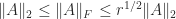 . The range space and null space of
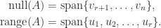

 rank-
rank- matrices, the
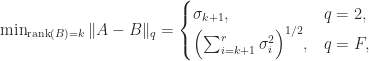

 terms gives the best rank-
 .
. ,
,  implies
 and
and  (modulo
  zeros in the latter case), and the singular vectors are eigenvectors. Moreover, the eigenvalues of the
  matrix
 additional zeros if
  , and the eigenvectors of
  can be expressed in terms of the SVD as
 , where
  is solved by
  , and when
  this is an underdetermined system and
  , where
  is orthogonal and
  is the polar decomposition and
  is unique. This connection between the SVD and the polar decomposition is useful both theoretically and computationally.