The spectral radius 


For Hermitian matrices (or more generally normal matrices, those satisfying 


Two classes of matrices for which the spectral radius is known are as follows.
- Unitary matrices (
): these have all their eigenvalues on the unit circle and so
.
- Nilpotent matrices (
for some positive integer
): such matrices have only zero eigenvalues, so
, even though
can be arbitrarily large.
The spectral radius of
Bounds
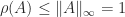
The spectral radius is bounded above by any consistent matrix norm (one satisfying 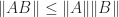

Theorem 1. For any

However, the spectral radius is not a norm and it can be zero when the 
Limit of Norms of Powers
The spectral radius can be expressed as a limit of norms of matrix powers.
Theorem 2 (Gelfand). For
.
The theorem implies that for large enough 


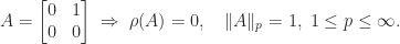
Spectral Radius of a Product
Little can be said about the spectral radius of a product of two matrices. The example
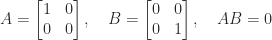
shows that we can have 

we have 
Condition Number Lower Bound
For a nonsingular matrix 

This bound can be very weak for nonnormal matrices.
Power Boundedness
In many situations we wish to know whether the powers of a matrix converge to zero. The spectral radius gives a necessary and sufficient condition for convergence.
Theorem 3. For
as
if and only if
.
The proof of Theorem 3 is straightforward if
Computing the Spectral Radius
Suppose 


In this pseudocode, norm(x) denotes the x.
Choose n-vector q_0 such that norm(q_0) = 1.
for k=1,2,...
    z_k = A q_{k-1}            % Apply A.
    q_k = z_k / norm(z_k)      % Normalize.
    mu_k = q_k^*Aq_k           % Rayleigh quotient.
end
The normalization is to avoid overflow and underflow and the 
If 
Here is an example where the power method converges quickly, thanks to the substantial ratio of 
>> rng(1); A = rand(4); eig_abs = abs(eig(A)), q = rand(4,1);
>> for k = 1:5, q = A*q; q = q/norm(q); mu = q'*A*q;
>>              fprintf('%1.0f %7.4e\n',k,mu)
>> end
eig_abs =
   1.3567e+00
   2.0898e-01
   2.5642e-01
   1.9492e-01
1 1.4068e+00
2 1.3559e+00
3 1.3580e+00
4 1.3567e+00
5 1.3567e+00
Nonnegative Matrices
For real matrices with nonnegative elements, much more is known about the spectral radius. Perron–Frobenius theory says that if 


rand function, which produces random matrices with elements on 
>> rng(1);  A = rand(4); e = sort(eig(A))
e =
  -2.0898e-01
   1.9492e-01
   2.5642e-01
   1.3567e+00
If 
![e = [1,1,\dots,1]^T](https://s0.wp.com/latex.php?latex=e+%3D+%5B1%2C1%2C%5Cdots%2C1%5D%5ET&bg=ffffff&fg=222222&s=0&c=20201002)

References
- Shmuel Friedland, Revisiting Matrix Squaring, Linear Algebra Appl., 154–156, 59-63, 1991.
- J. H. Wilkinson, The Algebraic Eigenvalue Problem, Oxford University Press, 1965, pp.~615–617.
Related Blog Posts
This article is part of the “What Is” series, available from https://nhigham.com/index-of-what-is-articles/ and in PDF form from the GitHub repository https://github.com/higham/what-is.
 upper Hessenberg matrix
  has the property that
  for
for  . For
. For  , the structure is
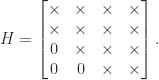
 flops. For example, the first stage of LU factorization needs to eliminate just one element, by adding a multiple of row
  ):
): 
 for all
  , then
  for any
  , which means that there is one linearly independent eigenvector associated with each eigenvalue of
  real parameters (the Schur parametrization), which are essentially the angles in the Givens QR factorization (note that in the QR factorization
  ,
,  is triangular and unitary and hence diagonal). The MATLAB function
  . For
. For  :
: 
 factor and the transpose of the
  factor in the LU factorization of tridiagonal matrices, and as the intermediate matrix in the computation of the singular value decomposition by the Golub–Reinsch algorithm.
  bidiagonal matrix:
 ![\notag \begin{bmatrix} a & x & 0 & 0 \\ & b & y & 0 \\ & & c & z \\ & & & d \end{bmatrix}^{-1} = \begin{bmatrix} \frac{1}{a} & -\frac{x}{a\,b} & \frac{x\,y}{a\,b\,c} & -\frac{x\,y\,z}{a\,b\,c\,d} \\[3pt] & \frac{1}{b} & -\frac{y}{b\,c} & \frac{y\,z}{b\,c\,d} \\[3pt] & & \frac{1}{c} & -\frac{z}{c\,d} \\[3pt] & & & \frac{1}{d} \end{bmatrix}.](https://s0.wp.com/latex.php?latex=%5Cnotag+%5Cbegin%7Bbmatrix%7D+a+++++++++++%26+x+++++++++++++++%26+0++++++++++++++++++++%26+0+%5C%5C+++++++++++++%26+b+++++++++++++++%26+y++++++++++++++++++++%26+0+%5C%5C+++++++++++++%26+++++++++++++++++%26+c++++++++++++++++++++%26+z+%5C%5C+++++++++++++%26+++++++++++++++++%26++++++++++++++++++++++%26+d+%5Cend%7Bbmatrix%7D%5E%7B-1%7D+%3D+%5Cbegin%7Bbmatrix%7D+%5Cfrac%7B1%7D%7Ba%7D+%26+-%5Cfrac%7Bx%7D%7Ba%5C%2Cb%7D+%26+%5Cfrac%7Bx%5C%2Cy%7D%7Ba%5C%2Cb%5C%2Cc%7D+%26+-%5Cfrac%7Bx%5C%2Cy%5C%2Cz%7D%7Ba%5C%2Cb%5C%2Cc%5C%2Cd%7D+%5C%5C%5B3pt%5D+++++++++++++%26+%5Cfrac%7B1%7D%7Bb%7D+++++%26+-%5Cfrac%7By%7D%7Bb%5C%2Cc%7D++++++%26+%5Cfrac%7By%5C%2Cz%7D%7Bb%5C%2Cc%5C%2Cd%7D++++++++%5C%5C%5B3pt%5D+++++++++++++%26+++++++++++++++++%26+%5Cfrac%7B1%7D%7Bc%7D++++++++++%26+-%5Cfrac%7Bz%7D%7Bc%5C%2Cd%7D+++++++++++++%5C%5C%5B3pt%5D+++++++++++++%26+++++++++++++++++%26++++++++++++++++++++++%26+%5Cfrac%7B1%7D%7Bd%7D+%5Cend%7Bbmatrix%7D.+&bg=ffffff&fg=222222&s=0&c=20201002)
 .
.  depend on
  , as there is no cancellation in the formulas for
  (less obvious, and provable by a scaling argument).
![f[\dots]](https://s0.wp.com/latex.php?latex=f%5B%5Cdots%5D&bg=ffffff&fg=222222&s=0&c=20201002) term is a divided difference.
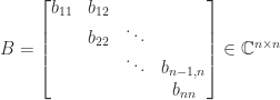
term is a divided difference.  is upper bidiagonal then
  is upper triangular with
  and
and ![\notag f_{ij} = b_{i,i+1} b_{i+1,i+2} \dots b_{j-1,j}\, f[b_{ii},b_{i+1,i+1}, \dots, b_{jj}], \quad j > i.](https://s0.wp.com/latex.php?latex=%5Cnotag+++++++f_%7Bij%7D+%3D+b_%7Bi%2Ci%2B1%7D+b_%7Bi%2B1%2Ci%2B2%7D+%5Cdots+b_%7Bj-1%2Cj%7D%5C%2C++++++++++++++++f%5Bb_%7Bii%7D%2Cb_%7Bi%2B1%2Ci%2B1%7D%2C+%5Cdots%2C+b_%7Bjj%7D%5D%2C+%5Cquad+j+%3E+i.+&bg=ffffff&fg=222222&s=0&c=20201002)
 Jordan block:
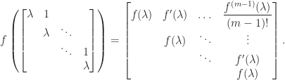
 in
in  to high accuracy in
 of
of  is an invariant subspace for
  if
if  , that is, if
  implies
  .
.  and
and  is an invariant subspace of
  implies
  .
. is a
is a 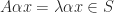 , where
 and a two-dimensional invariant subspace
  , where
  denotes the
  be linearly independent vectors. Then
 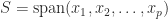 is an invariant subspace of
  for
for  . Writing
 ![X = [x_1,x_2,\dots,x_p]\in\mathbb{C}^{n \times p}](https://s0.wp.com/latex.php?latex=X+%3D+%5Bx_1%2Cx_2%2C%5Cdots%2Cx_p%5D%5Cin%5Cmathbb%7BC%7D%5E%7Bn+%5Ctimes+p%7D&bg=ffffff&fg=222222&s=0&c=20201002) , this condition can be expressed as
, this condition can be expressed as 
 .
.  in (1) then
  with
with  square and nonsingular, so
  , that is,
  the spectrum (set of eigenvalues) of
  the pseudoinverse of
  and
and  . Then
  . Furthermore, if
  is an eigenpair of
  then
then  is an eigenpair of
  is an eigenpair of
  , and
, and  since the columns of
  is an eigenpair of
  for some
  , and
, and  , since
  . Hence
 gives
gives  , so
, so  so that
 ![W = [X,\,Y]](https://s0.wp.com/latex.php?latex=W+%3D+%5BX%2C%5C%2CY%5D&bg=ffffff&fg=222222&s=0&c=20201002) is nonsingular. Let
is nonsingular. Let ![W^{-1} = \left[\begin{smallmatrix} G \\ H \end{smallmatrix}\right]](https://s0.wp.com/latex.php?latex=W%5E%7B-1%7D+%3D+%5Cleft%5B%5Cbegin%7Bsmallmatrix%7D+G+%5C%5C+H++++++++++++++++%5Cend%7Bsmallmatrix%7D%5Cright%5D&bg=ffffff&fg=222222&s=0&c=20201002) and note that
and note that  implies
  and
and  . We have
 ![\notag W^{-1}AW = \begin{bmatrix} G \\H \end{bmatrix} [AX,\, AY] = \begin{bmatrix} G \\H \end{bmatrix} [XB,\, AY] = \begin{bmatrix} B & GAY\\ 0 & HAY \end{bmatrix}, \qquad (2)](https://s0.wp.com/latex.php?latex=%5Cnotag++W%5E%7B-1%7DAW+%3D++%5Cbegin%7Bbmatrix%7D++++G+%5C%5CH++%5Cend%7Bbmatrix%7D+%5BAX%2C%5C%2C+AY%5D++%3D+%5Cbegin%7Bbmatrix%7D++++G+%5C%5CH++%5Cend%7Bbmatrix%7D+++%5BXB%2C%5C%2C+AY%5D++++%3D++%5Cbegin%7Bbmatrix%7D++++B+%26+GAY%5C%5C++++0+%26+HAY++%5Cend%7Bbmatrix%7D%2C+%5Cqquad+%282%29+&bg=ffffff&fg=222222&s=0&c=20201002)
 ,
,  chosen to be unitary.
  , where
  is unitary and
  and writing
 ![Q = [Q_1,\,Q_2]](https://s0.wp.com/latex.php?latex=Q+%3D+%5BQ_1%2C%5C%2CQ_2%5D&bg=ffffff&fg=222222&s=0&c=20201002) , where
, where  is
is  , and
, and 
 is
is  , we have
  . Hence
  matrix and let
  and
and  . Then the
  matrix
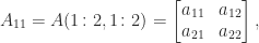
  is the submatrix of
  and the columns indexed by
  . For example, for the matrix
 ![\notag \begin{bmatrix} ~\fbox{1} & \fbox{2} & 3\mskip2mu \\ ~~4 & 5 & 6\mskip2mu~ \\ ~\fbox{7} & \fbox{8} & 9~\mskip2mu \end{bmatrix} = \begin{bmatrix} ~\fbox{1} & \fbox{2} & 3\mskip2mu~ \\[1pt] ~\fbox{4} & 5 & 6\mskip2mu~ \\ 7 & \fbox{8} & 9\mskip2mu \end{bmatrix},](https://s0.wp.com/latex.php?latex=%5Cnotag+++++%5Cbegin%7Bbmatrix%7D+%7E%5Cfbox%7B1%7D+%26+%5Cfbox%7B2%7D+%26+3%5Cmskip2mu+%5C%5C++++++++++++++++++++++++%7E%7E4+%26+5+%26+6%5Cmskip2mu%7E+%5C%5C++++++++++++++++++++++++%7E%5Cfbox%7B7%7D+%26+%5Cfbox%7B8%7D+%26+9%7E%5Cmskip2mu++++++++%5Cend%7Bbmatrix%7D+%3D+++++%5Cbegin%7Bbmatrix%7D+%7E%5Cfbox%7B1%7D+%26+%5Cfbox%7B2%7D+%26+3%5Cmskip2mu%7E+%5C%5C%5B1pt%5D++++++++++++++++++++++++%7E%5Cfbox%7B4%7D+%26+5+%26+6%5Cmskip2mu%7E+%5C%5C++++++++++++++++++++++++7+%26+%5Cfbox%7B8%7D+%26+9%5Cmskip2mu++++++++%5Cend%7Bbmatrix%7D%2C+&bg=ffffff&fg=222222&s=0&c=20201002)

 and columns
 matrix elements and the matrix itself, but there are many of intermediate size: an
  submatrices in total (counting both square and nonsquare submatrices).
  and
and  ,
,  , then
  ,
,  , then
  we denote by
  the sequence
  . Thus
  is another way of writing
  .
.  for the submatrix of
  to
to  , that is,

 denotes the
  the
the  matrix
  matrix, where each element is a
 ![\notag A = \left[\begin{array}{cc|cc} a_{11} & a_{12} & a_{13} & a_{14}\\ a_{21} & a_{22} & a_{23} & a_{24}\\\hline a_{31} & a_{32} & a_{33} & a_{34}\\ a_{41} & a_{42} & a_{43} & a_{44}\\ \end{array}\right] = \begin{bmatrix} A_{11} & A_{12} \\ A_{21} & A_{22} \end{bmatrix},](https://s0.wp.com/latex.php?latex=%5Cnotag+++A+%3D+%5Cleft%5B%5Cbegin%7Barray%7D%7Bcc%7Ccc%7D+++++++++a_%7B11%7D+%26+a_%7B12%7D+%26+a_%7B13%7D+%26+a_%7B14%7D%5C%5C+++++++++a_%7B21%7D+%26+a_%7B22%7D+%26+a_%7B23%7D+%26+a_%7B24%7D%5C%5C%5Chline+++++++++a_%7B31%7D+%26+a_%7B32%7D+%26+a_%7B33%7D+%26+a_%7B34%7D%5C%5C+++++++++a_%7B41%7D+%26+a_%7B42%7D+%26+a_%7B43%7D+%26+a_%7B44%7D%5C%5C+++++++++%5Cend%7Barray%7D%5Cright%5D++++%3D++%5Cbegin%7Bbmatrix%7D+++++++++A_%7B11%7D+%26+A_%7B12%7D+%5C%5C+++++++++A_%7B21%7D+%26+A_%7B22%7D++++++++%5Cend%7Bbmatrix%7D%2C+&bg=ffffff&fg=222222&s=0&c=20201002)
 ,
,  ,
,  ,
,  carried out on floating-point numbers. For example, evaluating the expression
  takes three flops. A square root, which occurs infrequently in numerical computation, is also counted as one flop.
  of two
  can be written
  additions, or
  of two
  inner products, costing
  flops. As we are usually interested in flop counts for large dimensions we retain only the highest order terms, so we regard
  flops.
  is a scalar,
  are
are  are
are 
 flops
flops
 flops
flops flops or less, so the interest is in the exponent (
 and comparing competing algorithms is more complicated.
  floating-point operations per second) for
 is the imaginary unit. Quaternions contain two more imaginary units,
  and
and  :
: 
 to “triplets”
  , but he realized that the requirement
  for the product of two such numbers could not hold. His key insight was to realize that a fourth imaginary unit,
  in general.
  Sir William Rowan Hamilton. Etching after J. Kirkwood. Credit: Wellcome Library, London. Wellcome Images.
  is an
is an  matrix
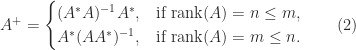
 .
. (overdetermined or underdetermined)
  minimizes
  and has the minimum
  is an SVD, where the
  are unitary and
  with
with  (so that
  ) with
  , then
 . This formula gives an easy way to prove many identities satisfied by the pseudoinverse. In MATLAB, the function
  and
and  .
.

 is
is  .
. ,
,  and if
  .
. is the transpose:
 for
for  . A sufficient condition for this equality to hold is that
  .
.
 as
as  . The convergence is at an asymptotically quadratic rate. However, about
  iterations are required to reach the asymptotic phase, where
  , so the iteration is slow to converge when
 is compact and convex (a nontrivial property proved by Toeplitz and Hausdorff), and it contains all the eigenvalues of
  matrices, with the eigenvalues shown as black dots. They were plotted using the function
 ,
,
 lies between the largest and smallest eigenvalues of the Hermitian matrix
  , which define a vertical strip in which the numerical range lies. Since
  , we can apply the same reasoning to the rotated matrix
  , and taking a range of
 ![\theta\in[0,\pi]](https://s0.wp.com/latex.php?latex=%5Ctheta%5Cin%5B0%2C%5Cpi%5D&bg=ffffff&fg=222222&s=0&c=20201002) we obtain an approximation the boundary of the numerical range.
we obtain an approximation the boundary of the numerical range.
 is the largest eigenvalue of the Hermitian matrix
  for small positive
  .
.
 . Also,
  , where
  is the spectral radius (the largest absolute value of any eigenvalue), since
 .
. does not hold in general). However, it is it true that

 then we can bound
  for all
 James Wilkinson’s 1963 book Rounding Errors in Algebraic Processes has been hugely influential. It came at a time when the effects of rounding errors on numerical computations in finite precision arithmetic had just starting to be understood, largely due to Wilkinson’s pioneering work over the previous two decades. The book gives a uniform treatment of error analysis of computations with polynomials and matrices and it is notable for making use of backward errors and condition numbers and thereby distinguishing problem sensitivity from the stability properties of any particular algorithm.
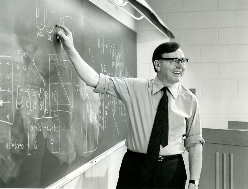
![[-1,1]](https://s0.wp.com/latex.php?latex=%5B-1%2C1%5D&bg=ffffff&fg=222222&s=0&c=20201002) with a fixed scale factor), and block floating-point arithmetic, which is a hybrid of floating-point arithmetic and fixed-point arithmetic. Although floating-point arithmetic dominates today’s computational landscape, fixed-point arithmetic is widely used in digital signal processing and block floating-point arithmetic is enjoying renewed interest in machine learning.
with a fixed scale factor), and block floating-point arithmetic, which is a hybrid of floating-point arithmetic and fixed-point arithmetic. Although floating-point arithmetic dominates today’s computational landscape, fixed-point arithmetic is widely used in digital signal processing and block floating-point arithmetic is enjoying renewed interest in machine learning.