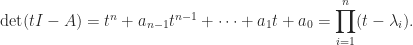
The determinant of an 


where the sum is over all 


The determinant is sometimes written with vertical bars, as 
Three fundamental properties are
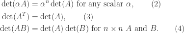
The first property is immediate, the second can be proved using properties of permutations, and the third is proved in texts on linear algebra and matrix theory.
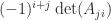
An alternative, recursive expression for the determinant is the Laplace expansion

for any 


For some types of matrices the determinant is easy to evaluate. If 
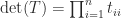


The determinant of 


For 

but already for 


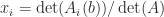
The determinant features in the formula

for the inverse, where 


Inequalities
A celebrated bound for the determinant of a Hermitian positive definite matrix 


Theorem 1 (Hadamard’s inequality). For a Hermitian positive definite matrix
with equality if and only if

Theorem 1 is easy to prove using a Cholesky factorization.
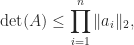
The following corollary can be obtained by applying Theorem 1 to 
Corollary 2. For
,
with equality if and only if the columns of
Obviously, one can apply the corollary to 
The determinant of 

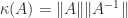
Nearness to Singularity and Conditioning
The determinant characterizes nonsingularity: 


To deal with the poor scaling one might normalize the determinant: in view of Corollary 2,
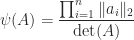
satisfies 


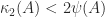


holds tends to 


>> rng(1); n = 50; A = randn(n);
>> psi = prod(sqrt(sum(A.*A)))/abs(det(A)), kappa2 = cond(A)
psi =
   5.3632e+10
kappa2 =
   1.5285e+02
>> ratio = psi/(n^(0.25)*exp(n/2))
ratio =
   2.8011e-01
The relative distance from
Theorem 3 (Gastinel, Kahan). For
and any subordinate matrix norm,

Notes
Determinants came before matrices, historically. Most linear algebra textbooks make significant use of determinants, but a lot can be done without them. Axler (1995) shows how the theory of eigenvalues can be developed without using determinants.
Determinants have little application in practical computations, but they are a useful theoretical tool in numerical analysis, particularly for proving nonsingularity.
There is a large number of formulas and identities for determinants. Sir Thomas Muir collected many of them in his five-volume magnum opus The Theory of Determinants in the Historical Order of Development, published between 1890 and 1930. Brualdi and Schneider (1983) give concise derivations of many identities using Gaussian elimination, bringing out connections between the identities.
The quantity obtained by modifying the definition (1) of determinant to remove the 


References
This is a minimal set of references, which contain further useful references within.
- Sheldon Axler, Down With Determinants!, Amer. Math. Monthly 102, 139–154, 1995.
- Garrett Birkhoff, Two Hadamard Numbers for Matrices, Comm. ACM 18, 25–29, 1975.
- Richard Brualdi and Hans Schneider, Determinantal Identities: Gauss, Schur, Cauchy, Sylvester, Kronecker, Jacobi, Binet, Laplace, Muir, and Cayley, Linear Algebra Appl. 52–53, 769–791, 1983.
- John Dixon, How Good is Hadamard’s Inequality for Determinants?, Canadian Math. Bulletin 27, 260–264, 1984.
- Alan Edelman, Eigenvalues and Condition Numbers of Random Matrices, SIAM J. Matrix Anal. Appl. 9(4), 543–560, 1988.
- Nicholas J. Higham, Accuracy and Stability of Numerical Algorithms, second edition, Society for Industrial and Applied Mathematics, Philadelphia, PA, USA, 2002.
Related Blog Posts
- The Strange Case of the Determinant of a Matrix of 1s and -1s by Nick Higham and Alan Edelman (2017)
- What Is a Vandermonde Matrix? (2021)
- What Is the Adjugate of a Matrix? (2020)
This article is part of the “What Is” series, available from https://nhigham.com/category/what-is and in PDF form from the GitHub repository https://github.com/higham/what-is.
