The 
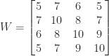
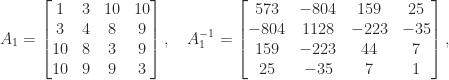
appears in a 1946 paper by Morris, in which it is described as having been “devised by Mr. T. S. Wilson.” The matrix is symmetric positive definite with determinant 
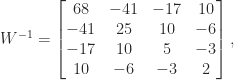
so it is moderately ill conditioned with 

Rutishauser (1968) stated that “the famous Wilson matrix is not a very striking example of an ill-conditioned matrix”, on the basis that 

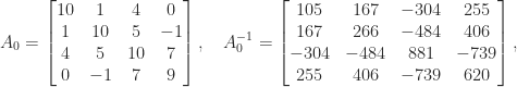
for which 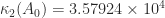

Moler (2018) asked how ill-conditioned
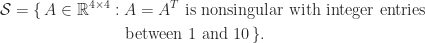
He generated one million random matrices from 
for which 
As the Wilson matrix is positive definite, we are also interested in how ill conditioned a matrix in the set

can be.
Condition Number Bounds
We first consider bounds on 


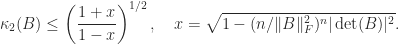
Applying this bound to 


Another result from Merikoski et al. (1997) gives, for symmetric positive definite 

For 


Recall that Rutishauser’s bound is 

Experiment
The sets 
- evaluates
from an explicit expression (exactly computed for such matrices) and discards
- computes the eigenvalues
of
(since
- for
The code is available at https://github.com/higham/wilson-opt.
The maximum over

which has 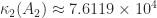

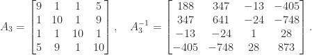
which has 
The following table summarizes the condition numbers of the matrices discussed and how close they are to the bounds.
| Matrix |
Comment | |
 |
 |
|---|---|---|---|---|
|
Wilson matrix |  |
99.73 | 13.40 |
 |
Rutishauser’s matrix |  |
8.31 | 1.12 |
 |
By random sampling |  |
6.19 | — |
 |
Optimal matrices in |
 |
3.91 | — |
 |
Optimal matrices in |
 |
8.38 | 1.13 |
Clearly, the bounds are reasonably sharp.
We do not know how Wilson constructed his matrix or to what extent he tried to maximize the condition number subject to the matrix entries being small integers. One possibility is that he constructed it via the factorization in the next section.
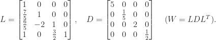
Integer Factorization
The Cholesky factor of the Wilson matrix is
![\notag R = \begin{bmatrix} \sqrt{5} & \frac{7\,\sqrt{5}}{5} & \frac{6\,\sqrt{5}}{5} & \sqrt{5}\\[\smallskipamount] 0 & \frac{\sqrt{5}}{5} & -\frac{2\,\sqrt{5}}{5} & 0\\[\smallskipamount] 0 & 0 & \sqrt{2} & \frac{3\,\sqrt{2}}{2}\\[\smallskipamount] 0 & 0 & 0 & \frac{\sqrt{2}}{2} \end{bmatrix} \quad (W = R^TR).](https://s0.wp.com/latex.php?latex=%5Cnotag+R+%3D+%5Cbegin%7Bbmatrix%7D+%5Csqrt%7B5%7D+%26+%5Cfrac%7B7%5C%2C%5Csqrt%7B5%7D%7D%7B5%7D+%26+%5Cfrac%7B6%5C%2C%5Csqrt%7B5%7D%7D%7B5%7D+%26+%5Csqrt%7B5%7D%5C%5C%5B%5Csmallskipamount%5D+0+%26+%5Cfrac%7B%5Csqrt%7B5%7D%7D%7B5%7D+%26+-%5Cfrac%7B2%5C%2C%5Csqrt%7B5%7D%7D%7B5%7D+%26+0%5C%5C%5B%5Csmallskipamount%5D+0+%26+0+%26+%5Csqrt%7B2%7D+%26+%5Cfrac%7B3%5C%2C%5Csqrt%7B2%7D%7D%7B2%7D%5C%5C%5B%5Csmallskipamount%5D+0+%26+0+%26+0+%26+%5Cfrac%7B%5Csqrt%7B2%7D%7D%7B2%7D+%5Cend%7Bbmatrix%7D+%5Cquad+%28W+%3D+R%5ETR%29.+&bg=ffffff&fg=222222&s=0&c=20201002)
Apart from the zero 

Suppose we drop the requirement of triangularity and ask whether the Wilson matrix has a factorization 


of 


The authors solve this equation computationally and find 
![\notag Z_1=\left[ \begin{array}{cccc} \frac{1}{2} & 1 & 0 & 1 \\ \frac{3}{2} & 2 & 3 & 3 \\ \frac{1}{2} & 1 & 0 & 0 \\ \frac{3}{2} & 2 & 1 & 0 \\ \end{array} \right], \quad Z_2=\left[ \begin{array}{@{\mskip2mu}rrrr} \frac{3}{2} & 2 & 2 & 2 \\ \frac{3}{2} & 2 & 2 & 1 \\ \frac{1}{2} & 1 & 1 & 2 \\ -\frac{1}{2} & -1 & 1 & 1 \\ \end{array} \right].](https://s0.wp.com/latex.php?latex=%5Cnotag+Z_1%3D%5Cleft%5B+%5Cbegin%7Barray%7D%7Bcccc%7D++%5Cfrac%7B1%7D%7B2%7D+%26+1+%26+0+%26+1+%5C%5C++%5Cfrac%7B3%7D%7B2%7D+%26+2+%26+3+%26+3+%5C%5C++%5Cfrac%7B1%7D%7B2%7D+%26+1+%26+0+%26+0+%5C%5C++%5Cfrac%7B3%7D%7B2%7D+%26+2+%26+1+%26+0+%5C%5C+%5Cend%7Barray%7D+%5Cright%5D%2C+%5Cquad+Z_2%3D%5Cleft%5B+%5Cbegin%7Barray%7D%7B%40%7B%5Cmskip2mu%7Drrrr%7D++%5Cfrac%7B3%7D%7B2%7D+%26+2+%26+2+%26+2+%5C%5C++%5Cfrac%7B3%7D%7B2%7D+%26+2+%26+2+%26+1+%5C%5C++%5Cfrac%7B1%7D%7B2%7D+%26+1+%26+1+%26+2+%5C%5C++-%5Cfrac%7B1%7D%7B2%7D+%26+-1+%26+1+%26+1+%5C%5C+%5Cend%7Barray%7D+%5Cright%5D.+&bg=ffffff&fg=222222&s=0&c=20201002)
They show that these matrices are the only factors 
Conclusions
The Wilson matrix has provided sterling service throughout the digital computer era as a convenient symmetric positive definite matrix for use in textbook examples and for testing algorithms. The recent discovery of its integer factorization has led to the development of new theory on when general 
Olga Taussky Todd wrote in 1961 that “matrices with integral elements have been studied for a very long time and an enormous number of problems arise, both theoretical and practical.” We wonder what else can be learned from the Wilson matrix and other integer test matrices.
References
This is a minimal set of references, which contain further useful references within.
- Nicholas J. Higham and Matthew C. Lettington, Optimizing and Factorizing the Wilson Matrix, to appear in Amer. Math. Monthly, 2021.
- Nicholas J. Higham, Matthew C. Lettington, and Karl Michael Schmidt, Integer Matrix Factorisations, Superalgebras and the Quadratic Form Obstruction, Linear Algebra Appl. 622, 250–267, 2021.
- Cleve B. Moler, Reviving Wilson’s Matrix, 2018.
- H. Rutishauser, On Test Matrices, 7 (no. 165), 349-365, in: Programmation en Mathematiques Numeriques, Besancon, 1968.
- Olga Taussky, Some Computational Problems Involving Integral Matrices, Journal of Research of the National Bureau of Standards Section B—Mathematical Sciences 65(1), 15–17, 1961.
Related Blog Posts
- What Is a Cholesky Factorization? (2020)
- What Is a Condition Number? (2020)
- What Is a Symmetric Positive Definite Matrix? (2020)
This article is part of the “What Is” series, available from https://nhigham.com/category/what-is and in PDF form from the GitHub repository https://github.com/higham/what-is.

Very interesting, Nick. Thanks. I especially like A_2. With all those 10s and 1s, you can feel the matrices pushing the boundaries. — Cleve
Thanks to Helmut Podhaisky for an improvement to the code at https://github.com/higham/wilson-opt to take advantage of the fact that we can assume without loss of generality that the diagonal is in nondecreasing order.