What Is a Totally Nonnegative Matrix?

The determinant of a square submatrix of a matrix is called a minor. A matrix $A\in\mathbb{R}^{n\times n}$ is totally positive if every minor is positive. It is totally nonnegative if every minor is nonnegative. These definitions require, in particular, that all the matrix elements must be nonnegative or positive, as must $\det(A)$ .

An important property is that total nonnegativity is preserved under matrix multiplication and hence under taking positive integer powers.

Theorem 1. If $A,B\in\mathbb{R}^{n\times n}$ are totally nonnegative then so is $AB$ .

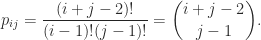
Theorem 1 is a direct consequence of the Binet–Cauchy theorem on determinants (also known as the Cauchy–Binet theorem). To state it, we need a way of specifying submatrices. We say the vector $\alpha = [\alpha_1,\alpha_2,\dots,\alpha_k]$ is an index vector of order $k$ if its components are integers from the set $\{1,2,\dots,n\}$ satisfying $\alpha_1 < \alpha_2 < \cdots < \alpha_k$ . If $\alpha$ and $\beta$ are index vectors of order $k$ and $\ell$ , respectively, then $A(\alpha, \beta)$ denotes the $k\times \ell$ matrix with ( $i,j$ ) element $a_{\alpha_i,\beta_j}$ .

Theorem 2. (Binet–Cauchy) Let $A\in\mathbb{R}^{m\times n}$ , $B\in\mathbb{R}^{n\times p}$ , and $C = AB$ . If $\alpha$ and $\beta$ are index vectors of order $k$ and $1 \le k \le \min(m,n,p)$ then

$\notag \det(C(\alpha,\beta)) = \sum_{\gamma} \det( A(\alpha,\gamma) ) \det( B(\gamma,\beta) ), \qquad (1)$

where the sum is over all index vectors $\gamma$ of order $k$ .

Note than when 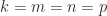$k = m = n = p$ , (1) reduces to the well-known relation $\det(AB) = \det(A)\det(B)$ , while when $k = 1$ , (1) reduces to the definition of matrix multiplication.

Totally nonnegative matrices have many interesting determinantal properties. For example, they satisfy Fischer’s inequality, first proved for symmetric positive definite matrices.

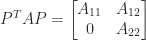
Theorem 3. (Fischer) If $A\in\mathbb{R}^{n\times n}$ is totally nonnegative then for any index vector $\alpha$ ,

$\notag \det(A) \le \det(A(\alpha)) \det(A(\alpha^c)), \qquad (2)$

where $\alpha^c$ comprises the indices not in $\alpha$ .

By repeatedly applying (2) with $\alpha$ containing just one element, we obtain Hadamard’s inequality for totally nonnegative $A$ :

$\notag \det(A) \le a_{11} a_{22} \cdots a_{nn}.$

Examples

We give some examples of totally positive matrices, showing how they can be generated in MATLAB. We use the Anymatrix toolbox.

A matrix well known to be positive definite, but which is also totally positive, is the Hilbert matrix $H\in\mathbb{R}^{n\times n}$ , with $h_{ij} = 1/(i+j-1)$ . The Hilbert matrix is a particular case of a Cauchy matrix $C$ , with $c_{ij} = 1/(x_i + y_j)$ for given vectors $x,y\in\mathbb{R}^{n\times n}$ . A Cauchy matrix is totally positive if $0 < x_1 < x_2 < \cdots < x_n$ and $0 < y_1 < y_2 < \cdots < y_n$ , which follows from the formula

$\notag \det(C_n) = \displaystyle\frac{\displaystyle\prod_{1\le i < j \le n} (x_j-x_i) (y_j-y_i) } {\displaystyle\prod_{1\le i,j \le n} (x_i+y_j) }.$

In MATLAB, the Hilbert matrix is hilb(n) and the Cauchy matrix can be generated by gallery('cauchy',x,y) (or anymatrix('gallery/cauchy',x,y)).

A Vandermonde matrix

$\notag V = V(x_1,x_2,\dots,x_n) = \begin{bmatrix} 1 & 1 & \dots & 1 \\ x_1 & x_2 & \dots & x_n \\ \vdots &\vdots & & \vdots \\ x_1^{n-1} & x_2^{n-1} & \dots & x_n^{n-1} \end{bmatrix} \in \mathbb{C}^{n\times n}$

is totally positive if the points $x_i$ satisfy $0 < x_1 < x_2 < \cdots < x_n$ . As a partial check, the general formula

$\notag \det(V) = \displaystyle\prod_{1\le i < j \le n}^n (x_i - x_j)$

shows that every leading principal minor is positive. In MATLAB, a Vandermonde matrix can be generated by anymatrix('core/vand',x).

The Pascal matrix $P_n\in\mathbb{R}^{n\times n}$ is defined by

$p_{ij} = \displaystyle\frac{ (i+j-2)! }{ (i-1)! (j-1)! } = {i+j-2 \choose j-1}.$

For example, in MATLAB:

>> P = pascal(5)
P =
     1     1     1     1     1
     1     2     3     4     5
     1     3     6    10    15
     1     4    10    20    35
     1     5    15    35    70

The Pascal matrix is totally positive for all $n$ (see the section below on bidiagonal factorizations).

The one-parameter correlation matrix $C_n(\theta)$ with off-diagonal elements given by $\theta$ with $0 \le \theta < 1$ , illustrated by

$\notag C_3(\theta) = \begin{bmatrix} 1 & \theta & \theta \\ \theta & 1 & \theta \\ \theta & \theta & 1 \\ \end{bmatrix},$

is not totally positive because while the principal minors are all positive, the submatrix $A([1,2],[2,3]) = \bigl[\begin{smallmatrix} \theta & \theta \\ 1 & \theta \end{smallmatrix}\bigr]$ has nonpositive determinant. However, the Kac–Murdock–Szegö matrix $K_n(\theta) = (\theta^{|i-j|})$ , with $0 \le \theta < 1$ , illustrated by

$\notag K_3(\theta) = \begin{bmatrix} 1 & \theta & \theta^2 \\ \theta & 1 & \theta \\ \theta^2 & \theta & 1 \\ \end{bmatrix}$

is totally positive thanks to the decay of the elements way from the diagonal. In MATLAB, the Kac–Murdock–Szegö matrix can be generated by gallery('kms',n,rho).

The lower Hessenberg Toeplitz matrix $H_n$ with all elements $1$ on and below the superdiagonal, illustrated for $n = 4$ by

$\notag H_4 = \begin{bmatrix} 1 & 1 & 0 & 0 \\ 1 & 1 & 1 & 0 \\ 1 & 1 & 1 & 1 \\ 1 & 1 & 1 & 1 \\ \end{bmatrix},$

is totally nonnegative. It has $\lfloor n/2 \rfloor$ zero eigenvalues, which appear in a single Jordan block, and its largest eigenvalue is $2(1+\cos(2\pi/(n+2)))$ . In MATLAB, this matrix can be generated by anymatrix('core/hessfull01',n). This and other binary totally nonnegative matrices are studied by Brualdi and Kirkland (2010).

Finally, consider a nonnegative $4\times 4$ bidiagonal matrix factorized into a product of elementary nonnegative bidiagonal matrices (nonnegative means that the elements of the matrix are nonnegative):

$\notag \begin{aligned} L = \begin{bmatrix} 1 & 0 & 0 & 0 \\ \ell_{21} & 1 & 0 & 0 \\ 0 & \ell_{32} & 1 & 0 \\ 0 & 9 & \ell_{43} & 1 \\ \end{bmatrix} &= \begin{bmatrix} 1 & 0 & 0 & 0 \\ \ell_{21} & 1 & 0 & 0 \\ 0 & 0 & 1 & 0 \\ 0 & 0 & 0 & 1 \\ \end{bmatrix} \begin{bmatrix} 1 & 0 & 0 & 0 \\ 0 & 1 & 0 & 0 \\ 0 & \ell_{32} & 1 & 0 \\ 0 & 0 & 0 & 1 \\ \end{bmatrix} \begin{bmatrix} 1 & 0 & 0 & 0 \\ 0 & 1 & 0 & 0 \\ 0 & 0 & 1 & 0 \\ 0 & 0 & \ell_{43} & 1 \\ \end{bmatrix}\\ &\equiv L_1(\ell_{21}) L_2(\ell_{32}) L_3(\ell_{43}). \end{aligned}$

It is easy to see by inspection that $L_1$ , $L_2$ , and $L_3$ are totally nonnegative, so $L$ is totally nonnegative by Theorem 1. With $D = \mathrm{diag}(1,-1,1,1,-1)$ , we have

$\notag \begin{aligned} DL^{-1}D &= (DLD)^{-1} = (DL_1D \cdot DL_2D \cdot DL_3D )^{-1}\\ &= (DL_3D)^{-1} (DL_2D)^{-1} (DL_3D)^{-1}\\ &= L_3(\ell_{43}) L_2(\ell_{32}) L_1(\ell_{21}), \qquad (3)\ \end{aligned}$

which is a product of totally nonnegative matrices and hence is totally nonnegative by Theorem 1. This example clearly generalizes to show that an $n\times n$ nonnegative bidiagonal matrix is totally nonnegative.

Inverse

Recall that the inverse of a nonsingular $A\in\mathbb{R}^{n\times n}$ is given by $A^{-1} = \mathrm{adj}(A)/\det(A)$ , where

$\mathrm{adj}(A) = \bigl( (-1)^{i+j} \det(A_{ji}) \bigr)$

and $A_{pq}$ denotes the submatrix of $A$ obtained by deleting row $p$ and column $q$ . If $A$ is nonsingular and totally nonnegative then it follows that $A^{-1}$ has a checkerboard (alternating) sign pattern. Indeed, we can write $A^{-1} = DBD$ , where $D = \mathrm{diag}((-1)^{i+1})$ and $B$ has nonnegative elements, and in fact it can be shown that $B$ is totally nonnegative using Theorem 1, Theorem 6, and (3). For example, here is the inverse of the $4\times 4$ Pascal matrix:

>> inv(sym(pascal(5)))
ans =
[  5, -10,  10,  -5,  1]
[-10,  30, -35,  19, -4]
[ 10, -35,  46, -27,  6]
[ -5,  19, -27,  17, -4]
[  1,  -4,   6,  -4,  1]

Eigensystem

A totally nonnegative matrix has nonnegative trace and determinant, so the sum and product of its eigenvalues are both nonnegative. In fact, all the eigenvalues are real and nonnegative. Since a Jordan block corresponding to a nonnegative eigenvalue is totally nonnegative any Jordan form with nonnegative eigenvalues is possible. More can be said of $A$ is irreducible. Recall that a matrix $A\in\mathbb{C}^{n\times n}$ is irreducible if there does not exist a permutation matrix $P$ such that

$\notag P^TAP = \begin{bmatrix} A_{11} & A_{12} \\ 0 & A_{22} \end{bmatrix}$

where $A_{11}$ and $A_{22}$ are square, nonempty submatrices.

Theorem 4. If $A\in\mathbb{R}^{n\times n}$ is totally nonnegative then its eigenvalues are all real and nonnegative. If $A$ is also irreducible then the positive eigenvalues are distinct.

If $A$ is nonsingular and totally nonnegative and irreducible then by the theorem we can write the eigenvalues as $\lambda_1 > \lambda_2 > \cdots > \lambda_n >0$ . It is known that the eigenvector $x_k$ associated with $\lambda_k$ has $k-1$ sign changes, that is, $(x_k)_{i+1}$ and ( $x_k)_i$ have opposite signs for $k-1$ values of $i$ (any zero elements are deleted before counting sign changes). Note that for $k=1$ , we already know from Perron–Frobenius theory that there is a positive eigenvector $x_1$ . This result is illustrated by the Pascal matrix above:

>> A = pascal(5); [V,d] = eig(A,'vector'); [~,k] = sort(d,'descend');
>> evals = d', evecs = V(:,k)
evals =
   1.0835e-02   1.8124e-01   1.0000e+00   5.5175e+00   9.2290e+01
evecs =
   1.7491e-02   2.4293e-01  -7.6605e-01  -5.7063e-01   1.6803e-01
   7.4918e-02   4.8079e-01  -3.8302e-01   5.5872e-01  -5.5168e-01
   2.0547e-01   6.1098e-01   1.6415e-01   2.5292e-01   7.0255e-01
   4.5154e-01   4.1303e-01   4.3774e-01  -5.1785e-01  -4.0710e-01
   8.6486e-01  -4.0736e-01  -2.1887e-01   1.7342e-01   9.0025e-02

Note that the number of sign changes (but not the number of negative elements) increases by $1$ as we go from one column to the next

The class of nonsingular totally nonnegative irreducible matrices is known as the oscillatory matrices, because such matrices arise in the analysis of small oscillations of elastic systems. An equivalent definition (in fact, the usual definition) is that an oscillatory matrix is a totally nonnegative matrix for which $A^q$ is totally positive for some positive integer $q$ .

LU Factorization

The next result shows that a totally nonnegative matrix has an LU factorization with special properties. We will need the following special case of Fischer’s inequality (Theorem 3):

$\notag \det(A) \le \det \bigl( A(1\colon p,1\colon p) \bigr) \det \bigl( A(p+1\colon n,p+1\colon n) \bigr), \quad p=1\colon n-1. \qquad (4)$

Theorem 5. If $A\in\mathbb{R}^{n\times n}$ is nonsingular and totally nonnegative then it has an LU factorization with $L$ and $U$ totally nonnegative and the growth factor $\rho_n = 1$ .

Proof. Since $A$ is nonsingular and every minor is nonnegative, (4) shows that $\det(A(1\colon p,1\colon p))>0$ for $p=1\colon n-1$ , which guarantees the existence of an LU factorization. That the elements of $L$ and $U$ are nonnegative follows from explicit determinantal formulas for the elements of $L$ and $U$ . The total nonnegativity of $L$ and $U$ is proved by Cryer (1976). Gaussian elimination starts with $A^{(1)} = A$ and computes $a_{ij}^{(k+1)} = a_{ij}^{(k)} - m_{ik}a_{kj}^{(k)} = a_{ij}^{(k)} - \ell_{ik} u_{kj} \le a_{ij}^{(k)}$ , since $\ell_{ik}, u_{kj} \ge 0$ . Thus $a_{ij} = a_{ij}^{(1)} \ge a_{ij}^{(2)} \ge \cdots \ge a_{ij}^{(r)}$ , $r = \min (i,j)$ . For $i > j$ , $a_{ij}^{(r)} \ge a_{ij}^{(r+1)} = \cdots = a_{ij}^{(n)} = 0$ ; for $j \ge i$ , $a_{ij}^{(r)} = \cdots = a_{ij}^{(n)} = u_{ij} \ge 0$ . Thus $0 \le a_{ij}^{(k)} \le a_{ij}$ for all $i,j,k$ and hence $\rho_n \le 1$ . But $\rho_n\ge1$ , so $\rho_n=1$ .

Theorem 5 implies that it is safe to compute the LU factorization without pivoting of a nonsingular totally nonnegativity matrix: the factorization does not break down and it is numerically stable. In fact, the computed LU factors have a strong componentwise form of stability. As shown by De Boor and Pinkus (1977), for small enough unit roundoff $u$ the computed factors $\widehat{L}$ and $\widehat{U}$ will have nonnegative elements and so from the standard backward error result for LU factorization,

$\notag \widehat{L}\widehat{U} = A + \Delta A, \quad |\Delta A| \le \gamma_n |\widehat{L}||\widehat{U}| \quad \Bigl(\gamma_n = \displaystyle\frac{nu}{1-nu} \Bigr),$

we have

$\notag |\widehat{L}||\widehat{U}| = |\widehat{L}\widehat{U}| = |A + \Delta A| \le |A| + \gamma_n |\widehat{L}||\widehat{U}|,$

which gives $|\widehat{L}||\widehat{U}| \le (1 - \gamma_n)^{-1}|A|$ and hence

$\notag \widehat{L}\widehat{U} = A + \Delta A, \quad |\Delta A| \le \displaystyle\frac{\gamma_n}{1-\gamma_n} |A|,$

which is about as strong a backward error result as we could hope for. The significance of this result is reduced, however, by the fact that for some important classes of totally nonnegative matrices, including Vandermonde matrices and Cauchy matrices, structure-exploiting linear system solvers exist that are substantially faster, and potentially more accurate, than LU factorization.

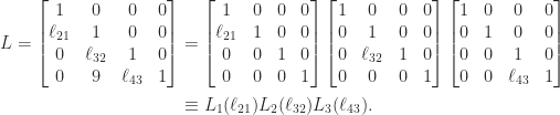
Factorization into a Product of Bidiagonal Matrices

We showed above that any nonnegative bidiagonal matrix is totally nonnegative. The next result shows that any nonsingular totally nonnegative matrix has an LU factorization in which $L$ and $U$ can be factorized into a product of nonnegative bidiagonal matrices.

Theorem 6. (Gasca and Peña, 1996) A nonsingular matrix $A\in\mathbb{R}^{n\times n}$ is totally nonnegative if and only if it it can be factorized as

$\notag A = L_{n-1} L_{n-2} \dots L_1 D U_1 U_2 \dots U_{n-1}, \qquad (5)$

where $D$ is a diagonal matrix with positive diagonal entries and $L_i$ and $U_i$ are unit lower and unit upper bidiagonal matrices, respectively, with the first $i-1$ entries along the subdiagonal of $L_i$ and $U_i^T$ zero and the rest nonnegative.

An analogue of Theorem 6 holds for totally positive matrices, the only difference being that the last $n-i+1$ subdiagonal entries of $L_i$ and $U_i^T$ are positive.

The factorization (5) can be computed by Neville elimination, which is a version of Gaussian elimination in which the eliminations are between adjacent rows, working from the bottom of each column upwards.

This factorization into bidiagonal factors can be used to obtain simple proofs of various properties of totally nonnegative matrices and totally positive matrices (Fallat, 2001). It also provides an efficient way to generates such matrices. If all the parameters in $D$ and the $L_i$ and $U_i$ are set to $1$ then the Pascal matrix is generated.

Testing for Total Positivity

An $n\times n$ matrix has $\sum_{i=1}^n {n \choose k} = 2^n-1$ principal minors (ones based on submatrices centred on the diagonal) and $\sum_{i=1}^n {n \choose k}^2 = {2n \choose n} -1 \approx 4^n/(n\pi)^{1/2}$ minors in total. However, it is not necessary to check all these minors to test for total positivity.

Theorem 7. (Gasca and Peña, 1996) The matrix $A\in\mathbb{R}^{n\times n}$ is totally positive if and only if $\det(A(\alpha,\beta)) > 0$ for all index vectors $\alpha$ and $\beta$ such that one of $\alpha$ and $\beta$ is $[1,2,\dots,k]$ and the entries of the other are $k$ consecutive integers.

Theorem 7 shows that only $n(n+1)$ minors need to be tested. Gasca and Peña have also show that total nonnegativity can be tested by checking about $2^{n+1} + n^2/2$ minors. A more efficient way to test for total nonnegativity is to compute the factorization in Theorem 6 and check the signs of the entries.

Notes

The results we have described show that totally nonnegative and totally positive matrices are analogous in many ways to symmetric positive (semi)definite matrices. The analogies go further because totally nonnegative and totally positive matrices also satisfy eigenvalue interlacing inequalities (albeit weaker than for symmetric matrices) and the eigenvalues of an oscillatory matrix majorize the diagonal elements. See Fallat and Johnson (2011) or Fallat (2014) for details.

References

This is a minimal set of references, which contain further useful references within.

Richard A. Brualdi and Steve Kirkland, Totally Nonnegative (0,1)-Matrices, Linear Algebra Appl. 432, 1650–1662, 2010.
Colin W. Cryer, Some Properties of Totally Positive Matrices, Linear Algebra Appl. 15, 1–25, 1976.
Carl de Boor and Allan Pinkus, Backward Error Analysis for Totally Positive Linear Systems, 27, 485–490, 1977.
Mariano Gasca and Juan M. Peña, On Factorizations of Totally Positive Matrices, in Mariano Gasca and Charles Micchelli, eds, Total Positivity and Its Applications, 109–130, Springer, 1996.
Shaun M. Fallat, Bidiagonal Factorizations of Totally Nonnegative Matrices, Amer. Math. Monthly 108 (6), 697–712, 2001.
Shaun M. Fallat, Totally Positive and Totally Nonnegative Matrices, in Handbook of Linear Algebra, Leslie Hogben, ed, 29.1–29.17, Chapman and Hall/CRC, 2014.
Shaun M. Fallat and Charles R. Johnson, Totally Nonnegative Matrices, Princeton University Press, Princeton, NJ, USA, 2011.

One thought on “What Is a Totally Nonnegative Matrix?”

José-Javier Martínez says:

July 27, 2021 at 10:47 am

Dear Professor Higham:

I am glad to see your new interesting post, with important references. However, your sentence “structure-exploiting linear system solvers exist that are substantially faster, and potentially more accurate” suggests a new one (useful not only for solving linear systems, but also for the computation of eigenvalues and singular values), a paper which has inspired a lot of work in this field:

-Plamen Koev: Accurate computations with totally nonnegative matrices. SIAM J. Matrix Anal. Appl. 29(3), pp. 731-751 (2007).
https://epubs.siam.org/doi/abs/10.1137/04061903X

Thank you for your wonderful work, and thank you also for giving the readers this freedom to add comments/complements.

What Is a Totally Nonnegative Matrix?

Examples

Inverse

Eigensystem

LU Factorization

Factorization into a Product of Bidiagonal Matrices

Testing for Total Positivity

Notes

References

Related Blog Posts

One thought on “What Is a Totally Nonnegative Matrix?”

Leave a comment Cancel reply

Examples

Inverse

Eigensystem

LU Factorization

Factorization into a Product of Bidiagonal Matrices

Testing for Total Positivity

Notes

References

Related Blog Posts

Share this:

Related

One thought on “What Is a Totally Nonnegative Matrix?”

Leave a comment Cancel reply