What Is a Matrix Norm?

A matrix norm is a function $\|\cdot\| : \mathbb{C}^{m\times n} \to \mathbb{R}$ satisfying

$\|A\| \ge 0$ with equality if and only if $A=0$ (nonnegativity),
$\|\alpha A\| =|\alpha| \|A\|$ for all $\alpha\in\mathbb{C}$ , $A\in\mathbb{C}^{m\times n}$ (homogeneity),
$\|A+B\| \le \|A\|+\|B\|$ for all $A,B\in\mathbb{C}^{m\times n}$ (the triangle inequality).

These are analogues of the defining properties of a vector norm.

An important class of matrix norms is the subordinate matrix norms. Given a vector norm on $\mathbb{C}^n$ the corresponding subordinate matrix norm on $\mathbb{C}^{m\times n}$ is defined by

$\notag \|A\| = \displaystyle\max_{x\ne0} \frac{ \|Ax\| }{ \|x\| },$

or, equivalently,

$\|A\| = \displaystyle\max_{\|x\| = 1} \|Ax\|.$

For the $1$ -, $2$ -, and $\infty$ -vector norms it can be shown that

$\notag \begin{alignedat}{2} \|A\|_1 &= \max_{1\le j\le n}\sum_{i=1}^m |a_{ij}|, &&\qquad \mbox{``max column sum'',} \\ \|A\|_{\infty} &= \max_{1\le i\le m}\sum_{j=1}^n |a_{ij}|, &&\qquad \mbox{``max row sum'',} \\ \|A\|_2 &= \sigma_{\max}(A), &&\qquad \mbox{spectral norm,} \end{alignedat}$

where $\sigma_{\max}(A)$ denotes the largest singular value of $A$ . To remember the formulas for the $1$ – and $\infty$ -norms, note that 1 is a vertical symbol (for columns) and $\infty$ is a horizontal symbol (for rows). For the general Hölder $p$ -norm no explicit formula is known for $\|A\|_p$ for $p\ne 1,2,\infty$ .

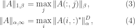
An immediate implication of the definition of subordinate matrix norm is that

$\notag \|AB\| \le \|A\| \|B\|$

whenever the product is defined. A norm satisfying this condition is called consistent or submultiplicative.

Another commonly used norm is the Frobenius norm,

$\notag \|A\|_F = \biggl( \displaystyle\sum_{i=1}^m \sum_{j=1}^n |a_{ij}|^2 \biggr)^{1/2} = \bigl( \mathrm{trace}(A^*\!A) \bigr)^{1/2}.$

The Frobenius norm is not subordinate to any vector norm (since $\|I_n\|_F = n^{1/2}$ , whereas $\|I_n\| = 1$ for any subordinate norm), but it is consistent.

The $2$ -norm and the Frobenius norm are unitarily invariant: they satisfy $\|UAV\| = \|A\|$ for any unitary matrices $U$ and $V$ . For the Frobenius norm the invariance follows easily from the trace formula.

As for vector norms, all matrix norms are equivalent in that any two norms differ from each other by at most a constant. This table shows the optimal constants $\alpha_{pq}$ such that $\|A\|_p \le \alpha_{pq} \|A\|_q$ for $A\in\mathbb{C}^{m\times n}$ and the norms mentioned above. Each inequality in the table is attained for some $A$ .

For any $A\in\mathbb{C}^{n\times n}$ and any consistent matrix norm,

$\notag \rho(A) \le \|A\|, \qquad\qquad (1)$

where $\rho$ is the spectral radius (the largest absolute value of any eigenvalue). To prove this inequality, let $\lambda$ be an eigenvalue of $A$ and $x$ the corresponding eigenvector (necessarily nonzero), and form the matrix $X=[x,x,\dots,x] \in \mathbb{C}^{n\times n}$ . Then $AX = \lambda X$ , so $|\lambda| \|X\| = \|AX\| \le \|A\| \, \|X\|$ , giving $|\lambda|\le\|A\|$ since $X \ne 0$ . For a subordinate norm it suffices to take norms in the equation $Ax = \lambda x$ .

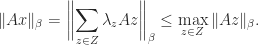
A useful relation is

$\notag \|A\|_2 \le \bigl( \|A\|_1 \|A\|_{\infty}\bigr)^{1/2}, \qquad\qquad (2)$

which follows from $\|A\|_2^2 = \|A^*A\|_2 = \rho(A^*A) \le \| A^*A \|_{\infty} \le \|A^*\|_{\infty} \|A\|_{\infty} = \|A\|_1 \|A\|_{\infty}$ , where the first two equalities are obtained from the singular value decomposition and we have used (1).

Mixed Subordinate Matrix Norms

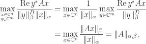
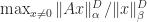
A more general subordinate matrix norm can be defined by taking different vector norms in the numerator and denominator:

$\notag \|A\|_{\alpha,\beta} = \displaystyle\max_{x\ne 0} \frac{ \|Ax\|_{\beta} }{ \|x\|_{\alpha} }.$

Some authors denote this norm by $\|A\|_{\alpha\to\beta}$ .

A useful characterization of $\|A\|_{\alpha,\beta}$ is given in the next result. Recall that $\|\cdot\|^D$ denotes the dual of the vector norm $\|\cdot\|$ .

Theorem 1. For $A\in\mathbb{C}^{m\times n}$ ,

$\notag \|A\|_{\alpha,\beta} = \displaystyle\max_{x\in\mathbb{C}^n \atop y \in\mathbb{C}^m} \frac{\mathrm{Re}\, y^*Ax}{\|y\|_\beta^D \|x\|_\alpha}.$

Proof. We have

$\notag \begin{aligned} \displaystyle \max_{x\in\mathbb{C}^n \atop y \in\mathbb{C}^m} \frac{\mathrm{Re}\, y^*Ax}{\|y\|_\beta^D \|x\|_\alpha} &= \max_{x\in\mathbb{C}^n} \frac{1}{\|x\|_\alpha} \max_{y\in\mathbb{C}^m} \frac{\mathrm{Re}\, y^*Ax}{\|y\|_\beta^D} \\ &= \max_{x\in\mathbb{C}^n} \frac{\| Ax \|_\beta }{\|x\|_\alpha} = \|A\|_{\alpha,\beta}, \end{aligned}$

where the second equality follows from the definition of dual vector norm and the fact that the dual of the dual norm is the original norm.

We can now obtain a connection between the norms of $A$ and $A^*$ . Here, $\|A^*\|_{\beta^D,\alpha^D}$ denotes $\max_{x\ne 0} \|Ax\|_\alpha^D / \|x\|_\beta^D$ .

Theorem 2. If $A\in\mathbb{C}^{m\times n}$ then $\|A\|_{\alpha,\beta} = \|A^*\|_{\beta^D,\alpha^D}$ .

Proof. Using Theorem 1, we have

$\notag \|A^*\|_{\alpha,\beta} = \displaystyle\max_{x\in\mathbb{C}^n \atop y \in\mathbb{C}^m} \frac{\mathrm{Re}\, y^*Ax}{\|y\|_\beta^D \|x\|_\alpha} = \displaystyle\max_{x\in\mathbb{C}^n \atop y \in\mathbb{C}^m} \frac{\mathrm{Re}\, x^*(A^*y)}{\|x\|_\alpha \|y\|_{\beta^D}} = \|A^*\|_{\beta^D,\alpha^D}. \quad\square$

If we take the $\alpha$ – and $\beta$ -norms to be the same $p$ -norm then we have $\|A\|_p = \|A^*\|_q$ , where $p^{-1} + q^{-1} = 1$ (giving, in particular, $\|A\|_2 = \|A^*\|_2$ and $\|A\|_1 = \|A^*\|_\infty$ , which are easily obtained directly).

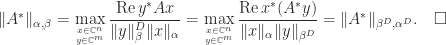
Now we give explicit formulas for the $(\alpha,\beta)$ norm when $\alpha$ or $\beta$ is $1$ or $\infty$ and the other is a general norm.

Theorem 3. For $A\in\mathbb{C}^{m\times n}$ ,

$\notag \begin{alignedat}{2} \|A\|_{1,\beta} &= \max_j \| A(:,j) \|_{\beta}, &\qquad\qquad& (3) \\ \|A\|_{\alpha,\infty} &= \max_i \|A(i,:)^*\|_{\alpha}^D, &\qquad\qquad& (4) \\ \end{alignedat}$

For $A\in\mathbb{R}^{m\times n}$ ,

$\notag \|A\|_{\infty,\beta} = \displaystyle\max_{x\in Z} \|Az\|_{\beta}, \qquad\qquad (5)$

where

$Z = \{ z\in\mathbb{R}^n: z_i = \pm 1~\mathrm{for~all}~i \,\},$

and if $A$ is symmetric positive semidefinite then

$\notag \|A\|_{\infty,1} = \displaystyle\max_{x\in Z} z^T\!Az.$

Proof. For (3),

$\notag \|Ax\|_{\beta} = \Big\| \sum_j x_j A(\colon,j) \Bigr\|_{\beta} \le \displaystyle\max_j \| A(\colon,j) \|_{\beta} \sum_j |x_j|,$

with equality for $x=e_k$ , where the maximum is attained for $j=k$ . For (4), using the Hölder inequality,

$\|Ax\|_{\infty} = \displaystyle\max_i | A(i,\colon) x | \le \max_i \bigl( \|A(i,\colon)^*\|_{\alpha}^D \|x\|_{\alpha} \bigr) = \|x\|_{\alpha} \max_i \|A(i,\colon)^*\|_{\alpha}^D.$

Equality is attained for an $x$ that gives equality in the Hölder inequality involving the $k$ th row of $A$ , where the maximum is attained for $i=k$ .

Turning to (5), we have $\|A\|_{\infty,\beta} = \max_{ \|x\|_\infty =1} \|Ax\|_\beta$ . The unit cube $\{\, x\in\mathbb{R}^n: -e \le x \le e\,\}$ , where $e = [1,1,\dots,1]^T$ , is a convex polyhedron, so any point within it is a convex combination of the vertices, which are the elements of $Z$ . Hence $\|x\|_\infty = 1$ implies

$\notag x = \displaystyle\sum_{z\in Z} \lambda_z Z, \quad \mathrm{where} \quad \lambda_z \ge 0, \quad \sum_{z\in Z} \lambda_z = 1$

and then

$\notag \|Ax\|_\beta = \biggl\| \displaystyle\sum_{z\in Z} \lambda_z Az \biggr\|_\beta \le \max_{z\in Z} \|Az\|_\beta.$

Hence $\max_{\|x\|_\infty = 1} \|Ax\|_\beta \le \max_{z\in Z} \|Az\|_\beta$ , but trivially $\max_{z\in Z} \|Az\|_\beta \le \max_{\|x\|_\infty = 1} \|Ax\|_\beta$ and (5) follows.

Finally, if $A$ is symmetric positive semidefinite let $\xi_z = \mathrm{sign}(Az) \in Z$ . Then, using a Cholesky factorization $A = R^T\!R$ (which exists even if $A$ is singular) and the Cauchy–Schwarz inequality,

$\notag \begin{aligned} \max_{z\in Z} \|Az\|_1 &= \max_{z\in Z} \xi_z^T Az = \max_{z\in Z} \xi_z^T R^T\!Rz\\ &= \max_{z\in Z} (R\xi_z)^T Rz \le \max_{z\in Z} \|R\xi_z\|_2 \|Rz\|_2\\ &\le \max_{z\in Z} \|Rz\|_2^2\\ &= \max_{z\in Z} z^T\!Az. \end{aligned}$

Conversely, for $z\in Z$ we have

$\notag z^T\!Az = |z^T\!Az| \le |z|^T|Az| = e^T |Az| = \|Az\|_1,$

so $\max_{z\in Z} z^T\!Az \le \max_{z\in Z} \|Az\|_1$ . Hence $\max_{z\in Z} z^T\!Az = \max_{z\in Z} \|Az\|_1 = \|A\|_{\infty,1}$ , using (5). $\square$

As special cases of (3) and (4) we have

$\notag \begin{aligned} \|A\|_{1,\infty} &= \max_{i,j} |a_{ij}|, \qquad\qquad\qquad (6) \\ \|A\|_{2,\infty} &= \max_i \|A(i,:)^*\|_2, \\ \|A\|_{1,2} &= \max_J \|A(:,j)\|_2. \end{aligned}$

We also obtain by using Theorem 2 and (5), for $A\in\mathbb{R}^{m\times n}$ ,

$\notag \|A\|_{2,1} = \displaystyle\max_{z\in Z} \|A^Tz\|_2.$

The $(2,\infty)$ -norm has recently found use in statistics (Cape, Tang, and Priebe, 2019), the motivation being that because it satisfies

$\notag \|A\|_{2,\infty} \le \|A\|_2 \le m^{1/2} \|A\|_{2,\infty},$

the $(2,\infty)$ -norm can be much smaller than the $2$ -norm when $m \gg n$ and so can be a better norm to use in bounds. The $(2,\infty)$ – and $(\infty,2)$ -norms are used by Rebrova and Vershynin (2018) in bounding the $2$ -norm of a random matrix after zeroing a submatrix. They note that the $2$ -norm of a random $n\times n$ matrix involves maximizing over infinitely many random variables, while the $(\infty,2)$ -norm and $(2,\infty)$ -norm involve only $2^n$ and $n$ random variables, respectively.

The ( $\alpha,\beta$ ) norm is not consistent, but for any vector norm $\gamma$ , we have

$\notag \begin{aligned} \|AB\|_{\alpha,\beta} &= \max_{x\ne0} \frac{ \|ABx\|_\beta }{ \|x\|_\alpha} = \max_{x\ne0} \frac{ \|A(Bx)\|_\beta }{ \|Bx\|_\gamma} \frac{ \|Bx\|_\gamma}{ \|x\|_\alpha} \le \max_{x\ne0} \frac{ \|A(Bx)\|_\beta }{ \|Bx\|_\gamma} \max_{x\ne0} \frac{ \|Bx\|_\gamma}{ \|x\|_\alpha}\\ &\le \|A\|_{\gamma,\beta} \|B\|_{\alpha,\gamma}. \end{aligned}$

Matrices With Constant $p$ -Norms

Let $A$ be a nonnegative square matrix whose row and column sums are all equal to $\mu$ . This class of matrices includes magic squares and doubly stochastic matrices. We have $\|A\|_1 = \|A\|_{\infty} = \mu$ , so $\|A\|_2 \le \mu$ by (2). But $Ae = \mu e$ for the vector $e$ of $1$ s, so $\mu$ is an eigenvalue of $A$ and hence $\|A\|_2 \ge \mu$ by (1). Hence $\|A\|_1 = \|A\|_2 = \|A\|_{\infty} = \mu$ . In fact, $\|A\|_p = \mu$ for all $p\in[1,\infty]$ (see Higham (2002, Prob. 6.4) and Stoer and Witzgall (1962)).

Computing Norms

The problem of computing or estimating $\|A\|_{\alpha,\beta}$ may be difficult for two reasons: we may not have an explicit formula for the norm, or $A$ may be given implicitly, as $A = f(B)$ , $A = B^{-1}$ , or $A = BC$ , for example, and we may wish to compute the norm without forming $A$ . Both difficulties are overcome by a generalization of the power method proposed by Tao in 1975 for arbitrary norms and independently Boyd in 1984 for $\alpha$ and $\beta$ both $p$ -norms (see Higham, 2002, Sec. $\,$ 15.2). The power method accesses $A$ only through matrix–vector products with $A$ and $A^*$ , so $A$ does not need to be explicitly available.

Let us focus on the case where $\alpha$ and $\beta$ are the same $p$ -norm. The power method is implemented in the Matrix Computation Toolbox as pnorm and we use it here to estimate the $\pi$ -norm and the $99$ -norm, which we compare with the $1$ -, $2$ -, and $\infty$ -norms.

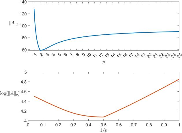
>> A = gallery('frank',4)
A =
     4     3     2     1
     3     3     2     1
     0     2     2     1
     0     0     1     1
>> [norm(A,1) norm(A,2) pnorm(A,pi), pnorm(A,99), norm(A,inf)]
ans =
   8.0000e+00   7.6237e+00   8.0714e+00   9.8716e+00   1.0000e+01

The plot in the top half of the following figure shows the estimated $p$ -norm for the matrix gallery('binomial',8) for $p \in[1,25]$ . This shape of curve is typical, because, as the plot in the lower half indicates, $\log(\|A\|_p)$ is a convex function of $1/p$ for $p\ge 1$ (see Higham, 2002, Sec. $\,$ 6.3).

The power method for the $(1,\infty)$ norm, which is the max norm in (6), is investigated by Higham and Relton (2016) and extended to estimate the $k$ largest values $a_{ij}$ or $|a_{ij}|$ .

A Norm Related to Grothendieck’s Inequality

A norm on $\mathbb{C}^{n\times n}$ can be defined by

$\notag \begin{aligned} \|A\|^{(t)} = \max \biggl\{ \bigg|\sum_{i,j=1}^n a_{ij} y^*_jx_i \bigg| : x_i,y_j \in\mathbb{C}^t, \; \|x_i\|_2 \le 1, \; \|y_j\|_2 \le 1, \; i,j=1\colon t \, \biggr\}. \end{aligned}$

Note that

$\notag \|A\|^{(1)} = \displaystyle\max_{0\ne x,y\in\mathbb{C}^n} \frac{|y^*Ax|}{\|y\|_\infty \|x\|_\infty} = \|A\|_{\infty,1}.$

A famous inequality of Grothendieck states that $\|A\|^{(n)} \le c \|A\|^{(1)}$ for all $A$ , for some constant $c$ independent of $n$ . Much work has been done to estimate the smallest possible constant $c$ , which is known to be in the interval $[1.33,1.41]$ , or $[1.67,1.79]$ for the analogous inequality for real data. See Friedland, Lim, and Zhang (2018) and the references therein.

Notes

The formula (5) with $\beta = 1$ is due to Rohn (2000), who shows that evaluating it is NP-hard. For general $\beta$ , the formula is given by Lewis (2010).

Computing mixed subordinate matrix norms based on $p$ -norms is generally NP-hard (Hendrickx and Olshevsky, 2010).

References

This is a minimal set of references, which contain further useful references within.

Joshua Cape, Minh Tang, and Carey Priebe, The Two-To-Infinity Norm and Singular Subspace Geometry with Applications to High-Dimensional Statistics, Ann. Statist. 47(5), 2405–2439, 2019.
Shmuel Friedland, Lek-Heng Lim and Jinjie Zhang, An Elementary and Unified Proof of Grothendieck’s Inequality, L’Enseignement Mathématique 64 (3), 327–351, 2018.
Julien Hendrickx and Alex Olshevsky, Matrix $p$ -Norms are NP-Hard to Approximate if $p\neq1,2,\infty$ , SIAM J. Matrix Anal. Appl. 31(5), 2802–2812, 2010.
Nicholas J. Higham, Accuracy and Stability of Numerical Algorithms, second edition, Society for Industrial and Applied Mathematics, Philadelphia, PA, USA, 2002.
Nicholas J. Higham and Samuel Relton, Estimating the Largest Elements of a Matrix, SIAM J. Sci. Comput. 38(5), C584–C601, 2016,
Andrew D. Lewis, A Top Nine List: Most Popular Induced Matrix Norms, Manuscript, 2010.
E. Rebrova and R. Vershynin, Norms of Random Matrices: Local and Global Problems, Adv. Math. 324, 40–83, 2018.
Josef Stoer and C. Witzgall, Transformations by Diagonal Matrices in a Normed Space, Numer. Math. 4(1), 158–171, 1962.

3 thoughts on “What Is a Matrix Norm?”

Daniel Kressner (@_kreda_) says:

October 13, 2021 at 8:48 am

Thanks, Nick, this is a great summary!

yasir says:

October 22, 2022 at 6:41 pm

Sir, how could we compute L-1/L-infinity Mixed induced matrix norms?

1. Nick Higham says:
  
  October 22, 2022 at 7:12 pm
  
  By (3) it is $\max_{i,j} |a_{ij}|$.

What Is a Matrix Norm?

Mixed Subordinate Matrix Norms

Matrices With Constant $p$ -Norms

Computing Norms

A Norm Related to Grothendieck’s Inequality

Notes

References

Related Blog Posts

3 thoughts on “What Is a Matrix Norm?”

Leave a Reply Cancel reply

Mixed Subordinate Matrix Norms

Matrices With Constant -Norms

Computing Norms

A Norm Related to Grothendieck’s Inequality

Notes

References

Related Blog Posts

Share this:

Related

3 thoughts on “What Is a Matrix Norm?”

Leave a Reply Cancel reply

Matrices With Constant $p$ -Norms