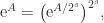
The exponential of a square matrix 

That the series converges follows from the convergence of the series for scalars. Various other formulas are available, such as

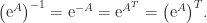
The matrix exponential is always nonsingular and 
Much interest lies in the connection between 


![[A,B] = AB - BA](https://s0.wp.com/latex.php?latex=%5BA%2CB%5D+%3D+AB+-+BA&bg=ffffff&fg=222222&s=0&c=20201002)

Especially important is the relation
for integer 
Another important property of the matrix exponential is that it maps skew-symmetric matrices to orthogonal ones. Indeed if 
This is a special case of the fact that the exponential maps elements of a Lie algebra into the corresponding Lie group.
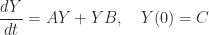
The matrix exponential plays a fundamental role in linear ordinary differential equations (ODEs). The vector ODE

has solution 

is 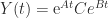
In control theory, the matrix exponential is used in converting from continuous time dynamical systems to discrete time ones. Another application of the matrix exponential is in centrality measures for nodes in networks.
Many methods have been proposed for computing the matrix exponential. See the references for details.
References
This is a minimal set of references, which contain further useful references within.
- Awad H. Al-Mohy and Nicholas J. Higham, A New Scaling and Squaring Algorithm for the Matrix Exponential, SIAM J. Matrix Anal. Appl. 31(3), 970–989, 2009.
- Ernesto Estrada and Philip A. Knight, A First Course in Network Theory, Oxford University Press, 2015.
- Nicholas J. Higham, Functions of Matrices: Theory and Computation, Society for Industrial and Applied Mathematics, Philadelphia, PA, USA, 2008. (Chapter 10).
- Cleve B. Moler and Van Loan, Charles F., Nineteen Dubious Ways to Compute the Exponential of a Matrix, Twenty-Five years Later, SIAM Rev. 45(1), 3–49, 2003.
- Gilbert Strang, The Matrix Exponential (video), 2016.
Related Blog Posts
- A Balancing Act for the Matrix Exponential by Cleve Moler (2012)
- The Improved MATLAB Functions Expm and Logm (2016)
- Update of Catalogue of Software for Matrix Functions (2020)
This article is part of the “What Is” series, available from https://nhigham.com/category/what-is and in PDF form from the GitHub repository https://github.com/higham/what-is.

 .
. -by-
-by- floating-point operations, each of which needs to be chopped. The following code uses only
  calls to
  matrix
  such that
  .
. (
( ), there are two square roots (which are equal if
  ), and they are real if and only if
  , depending on the matrix there can be no square roots, finitely many, or infinitely many. The matrix
 . The identity matrix
 involutory matrices), including
  , the lower triangular matrix
![\begin{bmatrix} \cos \theta & \sin \theta \\ \sin \theta & -\cos \theta \end{bmatrix}, \quad \theta \in[0,2\pi]](https://s0.wp.com/latex.php?latex=%5Cbegin%7Bbmatrix%7D++++++%5Ccos+%5Ctheta++%26++%5Csin+%5Ctheta+%5C%5C++++++%5Csin+%5Ctheta++%26+-%5Ccos+%5Ctheta++++++%5Cend%7Bbmatrix%7D%2C+%5Cquad+%5Ctheta+%5Cin%5B0%2C2%5Cpi%5D+&bg=ffffff&fg=222222&s=0&c=20201002)
 . If
. If  above,
  .
. , where
  is orthogonal and
  is also symmetric positive definite.
 square roots, where
  such that
  is called a square root, but this is not the standard meaning.
 -matrices,
![G(\theta) = \begin{bmatrix} \cos \theta & \sin \theta \\ -\sin \theta & \cos \theta \end{bmatrix}, \quad \theta \in[0,2\pi],](https://s0.wp.com/latex.php?latex=G%28%5Ctheta%29+%3D+%5Cbegin%7Bbmatrix%7D++++++%5Ccos+%5Ctheta++%26++%5Csin+%5Ctheta+%5C%5C++++++-%5Csin+%5Ctheta++%26+%5Ccos+%5Ctheta++++++%5Cend%7Bbmatrix%7D%2C+%5Cquad+%5Ctheta+%5Cin%5B0%2C2%5Cpi%5D%2C+&bg=ffffff&fg=222222&s=0&c=20201002)
 radians clockwise. The natural square root of
  is
is  . For
. For  , this gives the square root
 th roots of stochastic matrices


 , as can be seen by taking norms, so let us concentrate on the smallest singular value.
 , for unit norm
  and
and  . The matrix
  times) and
  . The matrix is singular—and hence has a zero singular value—precisely when
  , which is the smallest value that the inner product
  can take.
 , where
  and
and  is singular with null vector
  , which is the identity plus a rank-
 singular values remain at 1.
 and
and  respectively! As our example shows,
  and
and  to be unit-norm random vectors with independent entries from the same distribution.
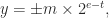
 is the precision and
 ![e\in [e_{\min},e_{\max}]](https://s0.wp.com/latex.php?latex=e%5Cin+%5Be_%7B%5Cmin%7D%2Ce_%7B%5Cmax%7D%5D&bg=ffffff&fg=222222&s=0&c=20201002) is the exponent. The significand
is the exponent. The significand  is an integer satisfying
  . Numbers with
  are called normalized. Subnormal numbers, for which
  and
and  , are supported.
 .
.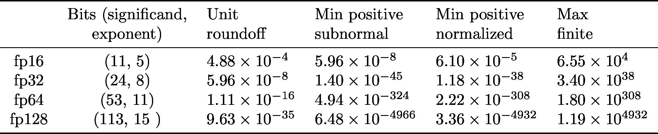 Fp32 (single precision) and fp64 (double precision) were in the 1985 standard; fp16 (half precision) and fp128 (quadruple precision) were introduced in 2008. Fp16 is defined only as a storage format, though it is widely used for computation.
 (usually written as inf in programing languages) as floating-point numbers: every arithmetic operation produces a number in the system. A NaN is generated by operations such as

 evaluates as
  when
when  .
.
 denotes the computed result. The standard also includes a fused multiply-add operation (FMA),
  . The definition requires it to be computed with just one rounding error, so that
  is the rounded version of
  , and hence satisfies
 ) and transcendental functions (
 ,
,  ,
,  ,
,  , etc.) and defines domains and special values for them, but these functions are not required.
 along with the error
  , for
, for  . These operations are useful for implementing compensated summation and other special high accuracy algorithms.
 is a finite subset of the real line comprising numbers of the form
 is the base,
  , and
, and  . The significand
 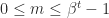 . Normalized numbers are those for which
  , and they have a unique representation. Subnormal numbers are those with
  and
and  is
is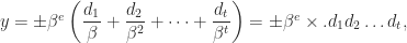
 satisfies
 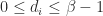 and
and  for normalized numbers.
 ,
,  , and
, and ![e \in [-1, 3]](https://s0.wp.com/latex.php?latex=e+%5Cin+%5B-1%2C+3%5D&bg=ffffff&fg=222222&s=0&c=20201002) .
.
 and
and  , which is called the machine epsilon. Note that
  .
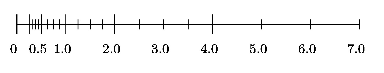
. and the smallest normalized number, which is
  . The subnormal numbers fill this gap with numbers having the same spacing as those between
  , namely
  . The next diagram shows the complete set of nonnegative normalized and subnormal numbers in the toy system.
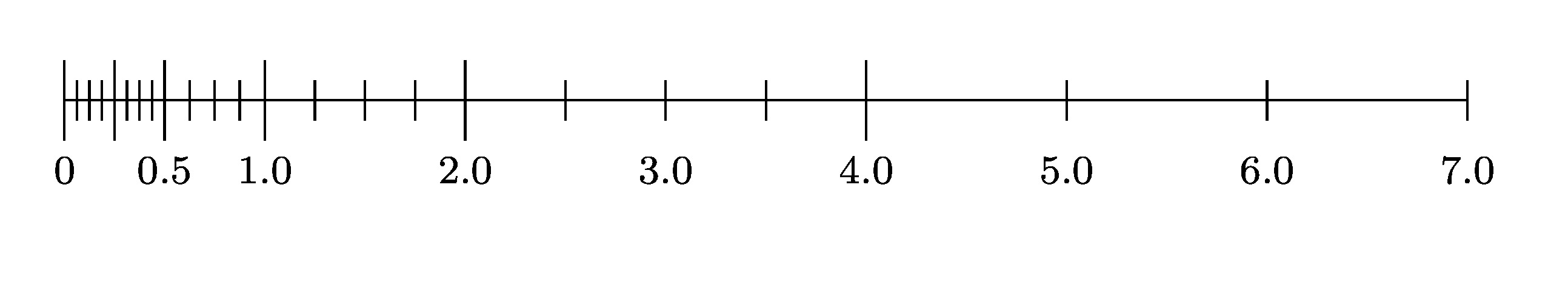
 . If
. If  then
then  ; otherwise,
  and
and  then
then 
 ,
,  ,
,  ,
,  , and
, and  are usually defined to return the correctly rounded exact result, so they satisfy
 , so all the numbers are equally spaced. In most scientific computations scale factors must be introduced in order to be able to represent the range of numbers occurring. Fixed-point arithmetic is mainly used on special purpose devices such as FPGAs and in embedded systems.