What Is the Trace of a Matrix?

The trace of an $n\times n$ matrix is the sum of its diagonal elements: $\mathrm{trace}(A) = \sum_{i=1}^n a_{ii}$ . The trace is linear, that is, $\mathrm{trace}(A+B) = \mathrm{trace}(A) + \mathrm{trace}(B)$ , and $\mathrm{trace}(A) = \mathrm{trace}(A^T)$ .

A key fact is that the trace is also the sum of the eigenvalues. The proof is by considering the characteristic polynomial $p(t) = \det(t I - A) = t^n + a_{n-1}t^{n-1} + \dots + a_1 t + a_0$ . The roots of $p$ are the eigenvalues $\lambda_1, \lambda_2, \dots, \lambda_n$ of $A$ , so $p$ can be factorized

$\notag p(t) = (t - \lambda_1) (t - \lambda_2) \dots (t - \lambda_n),$

and so $a_{n-1} = -(\lambda_1 + \lambda_2 + \cdots + \lambda_n)$ . The Laplace expansion of $\det(t I - A)$ shows that the coefficient of $t^{n-1}$ is $-(a_{11} + a_{22} + \cdots + a_{nn})$ . Equating these two expressions for $a_{n-1}$ gives

$\notag \mathrm{trace}(A) = \displaystyle\sum_{i=1}^n \lambda_i. \qquad\qquad(1)$

A consequence of (1) is that any transformation that preserves the eigenvalues preserves the trace. Therefore the trace is unchanged under similarity transformations: $\mathrm{trace}(X^{-1}AX) = \mathrm{trace}(A)$ for any nonsingular $X$ .

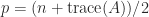
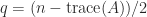
An an example of how the trace can be useful, suppose $A$ is a symmetric and orthogonal $n\times n$ matrix, so that its eigenvalues are $\pm 1$ . If there are $p$ eigenvalues $1$ and $q$ eigenvalues $-1$ then $\mathrm{trace}(A) = p - q$ and $n = p + q$ . Therefore $p = (n + \mathrm{trace}(A))/2$ and $q = (n - \mathrm{trace}(A))/2$ .

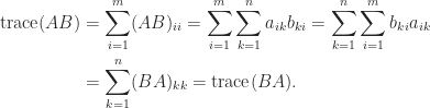
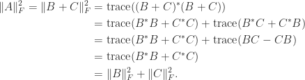
Another important property is that for an $m\times n$ matrix $A$ and an $n\times m$ matrix $B$ ,

$\notag \mathrm{trace}(AB) = \mathrm{trace}(BA) \qquad\qquad(2)$

(despite the fact that $AB \ne BA$ in general). The proof is simple:

$\notag \begin{aligned} \mathrm{trace}(AB) &= \displaystyle\sum_{i=1}^m (AB)_{ii} = \sum_{i=1}^m \sum_{k=1}^n a_{ik} b_{ki} = \sum_{k=1}^n \sum_{i=1}^m b_{ki} a_{ik} \\ & = \sum_{k=1}^n (BA)_{kk} = \mathrm{trace}(BA). \end{aligned}$

This simple fact can have non-obvious consequences. For example, consider the equation $AX - XA = I$ in $n\times n$ matrices. Taking the trace gives $0 = \mathrm{trace}(AX) - \mathrm{trace}(XA) = \mathrm{trace}(AX - XA) = \mathrm{trace}(I) = n$ , which is a contradiction. Therefore the equation has no solution.

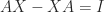
The relation (2) gives $\mathrm{trace}(ABC) = \mathrm{trace}((AB)C) = \mathrm{trace}(C(AB)) = \mathrm{trace}(CAB)$ for $n\times n$ matrices $A$ , $B$ , and $C$ , that is,

$\notag \mathrm{trace}(ABC) = \mathrm{trace}(CAB). \qquad\qquad(3)$

So we can cyclically permute terms in a matrix product without changing the trace.

As an example of the use of (2) and (3), if $x$ and $y$ are $n$ -vectors then $\mathrm{trace}(xy^T) = \mathrm{trace}(y^Tx) = y^Tx$ . If $A$ is an $n\times n$ matrix then $\mathrm{trace}(xy^TA)$ can be evaluated without forming the matrix $xy^TA$ since, by (3), $\mathrm{trace}(xy^TA) = \mathrm{trace}(y^TAx) = y^TAx$ .

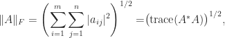
The trace is useful in calculations with the Frobenius norm of an $m\times n$ matrix:

$\notag \|A\|_F = \left(\displaystyle\sum_{i=1}^m \sum_{j=1}^n |a_{ij}|^2\right)^{1/2} = \bigr(\mathrm{trace}(A^*A)\bigr)^{1/2},$

where $*$ denotes the conjugate transpose. For example, we can generalize the formula $|x+\mathrm{i}y|^2 = x^2 + y^2$ for a complex number to an $m\times n$ matrix $A$ by splitting $A$ into its Hermitian and skew-Hermitian parts:

$\notag A = \frac{1}{2}(A+A^*) + \frac{1}{2}(A-A^*) \equiv B + C,$

where $B = B^*$ and $C = -C^*$ . Then

$\notag \begin{aligned} \|A\|_F^2 = \|B + C\|_F^2 &= \mathrm{trace}((B+C)^*(B+C))\\ &= \mathrm{trace}(B^*B + C^*C) + \mathrm{trace}(B^*C + C^*B)\\ &= \mathrm{trace}(B^*B + C^*C) + \mathrm{trace}(BC - CB)\\ &= \mathrm{trace}(B^*B + C^*C)\\ &= \|B\|_F^2 + \|C\|_F^2. \end{aligned}$

If a matrix is not explicitly known but we can compute matrix–vector products with it then the trace can be estimated by

$\notag \mathrm{trace}(A) \approx x^TAx,$

where the vector $x$ has elements independently drawn from the standard normal distribution with mean $0$ and variance $1$ . The expectation of this estimate is

$\notag \begin{aligned} E\bigl( x^TAx \bigr) &= E\bigl( \mathrm{trace}(x^TAx) \bigr) = E\bigl( \mathrm{trace}(Axx^T) \bigr) = \mathrm{trace} \bigl( E(Axx^T) \bigr) \\ &= \mathrm{trace}\bigl(A E(xx^T) \bigr) = \mathrm{trace}(A), \end{aligned}$

since $E(x_ix_j) = 0$ for $i\ne j$ and $E(x_i^2) = 1$ for all $i$ , so $E(xx^T) = I$ . This stochastic estimate, which is due to Hutchinson, is therefore unbiased.