What Is a Rank-Revealing Factorization?

In many applications a matrix A\in\mathbb{R}^{m\times n} has less than full rank, that is, r = \mathrm{rank}(A) < \min(m,n). Sometimes, r is known, and a full-rank factorization A = GH with G\in\mathbb{R}^{m \times r} and H\in\mathbb{R}^{r \times n}, both of rank r, is given—especially when r = 1 or r = 2. Often, though, the rank r is not known. Moreover, rather than being of exact rank r, A is merely close to a rank r matrix because of errors from various possible sources.

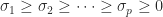
What is usually wanted is a factorization that displays how close
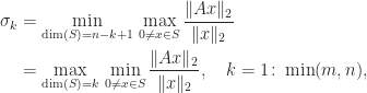
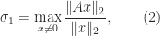
 A is to having particular ranks and provides an approximation to the range space of a lower rank matrix. The ultimate tool for providing this information is the singular value decomposition (SVD)

\notag     A = U\Sigma V^T, \quad    \Sigma = \mathrm{diag}(\sigma_1,\dots, \sigma_p)\in\mathbb{R}^{m\times n},

where p = \min(m,n), \sigma_1\ge \sigma_2\ge \cdots \ge \sigma_p \ge 0, and U\in\mathbb{R}^{m\times m} and V\in\mathbb{R}^{n\times n} are orthogonal. The Eckart–Young theorem says that

\notag  \min_{\mathrm{rank}(B) = k} \|A-B\|_q =  \begin{cases}      \sigma_{k+1},                                & q = 2,  \\      \Bigl(\sum_{i=k+1}^r \sigma_i^2\Bigr)^{1/2}, & q = F,   \end{cases}

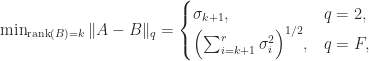
and that the minimum is attained at

\notag    A_k = U \Sigma_k V^T, \quad    \Sigma_k = \mathrm{diag}(\sigma_1, \dots, \sigma_k, 0, \dots, 0),

so A_k is the best rank-k approximation to A in both the 2-norm and the Frobenius norm.

Although the SVD is expensive to compute, it may not be significantly more expensive than alternative factorizations. However, the SVD is expensive to update when a row or column is added to or removed from the matrix, as happens repeatedly in signal processing applications.

Many different definitions of a rank-revealing factorization have been given, and they usually depend on a particular matrix factorization. We will use the following general definition.

Definition 1. A rank-revealing factorization (RRF) of A\in\mathbb{R}^{m\times n} is a factorization

\notag   A = XDY^T, \quad   X\in\mathbb{R}^{m\times p}, \quad   D\in\mathbb{R}^{p\times p}, \quad   Y\in\mathbb{R}^{n\times p},

where p \le \min(m,n), D is diagonal and nonsingular, and X and Y are well conditioned.

An RRF concentrates the rank deficiency and ill condition of A into the diagonal matrix D. An RRF clearly exists, because the SVD is one, with X and Y having orthonormal columns and hence being perfectly conditioned. Justification for this definition comes from a version of Ostrowski’s theorem, which shows that

\notag     \sigma_i(A) = \theta_i \sigma_i(D), \quad i = 1\colon \min(m,n),      \qquad (1)

where \sigma_p(X)\sigma_p(Y) \le \theta_i \le \sigma_1(X) \sigma_1(Y). Hence as long as X and Y are well conditioned, the singular values are good order of magnitude approximations to those of A up a scale factor.

Without loss of generality we can assume that

\notag   D = \mathrm{diag}(d_i), \quad   |d_1| \ge |d_2| \ge \cdots \ge |d_p|

(since XDY^T = XP\cdot P^TDP \cdot P^T Y^T for any permutation matrix P and the second expression is another RRF). For \widetilde{A}_k = X \mathrm{diag}(d_1,\dots,d_k,0,\dots,0)Y^T we have

\notag   \|A - \widetilde{A}_k\| \le \|X\| \|Y\|   \|\mathrm{diag}(0,\dots,0,d_{k+1},\dots,d_p)\|,

so A is within distance of order |d_{k+1}| from the rank-k matrix \widetilde{A}_k, which is the same order as the distance to the nearest rank-k matrix if |d_{k+1}| \approx \sigma_{k+1}.

Definition 2 is a strong requirement, since it requires all the singular values of A to be well approximated by the (scaled) diagonal elements of D. We will investigate below how it compares with another definition of RRF.

Numerical Rank

An RRF helps to determine the numerical rank, which we now define.

Definition 2. For a given \epsilon > 0 the numerical rank of A is the largest integer k such that \sigma_k > \epsilon.

By the Eckart–Young theorem, the numerical rank is the smallest rank attained over all A+E with \|E\|_2 \le \epsilon. For the numerical rank to be meaningful in the sense that it is unchanged if \epsilon is perturbed slightly, we need \epsilon not to be too close to \sigma_k or \sigma_{k+1}, which means that there must be a significant gap between these two singular values.

QR Factorization

One might attempt to compute an RRF by using a QR factorization A = QR, where Q\in\mathbb{R}^{m\times n} has orthonormal columns, R\in\mathbb{R}^{n\times n} is upper triangular, and we assume that m\ge n. In Definition 1, we can take

\notag   X = I, \quad D = \mathrm{diag}(R), \quad Y^T = D^{-1}R. \qquad (*)

However, it is easy to see that QR factorization in its basic form is flawed as a means for computing an RRF. Consider the matrix

\notag   A = \begin{bmatrix}        0 & 1  & 0 &0\\        0 & 0  & 1 &0 \\        0 & 0  & 0 &1\\        0 & 0  & 0 &0   \end{bmatrix},

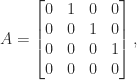
which is a Jordan block with zero eigenvalue. This matrix is its own QR factorization (R = A), and the prescription (*) gives D = 0, so A \ne XDY^T. The essential problem is that the diagonal of R has no connection with the nonzero singular values of A. What is needed are column permutations: A\Pi = \mathrm{diag}(1,1,1,0) for the permutation matrix \Pi that reorders [a_1,a_2,a_3,a_4] to [a_2,a_3,a_4,a_1], and this is a perfect RRF with X = Y = I.

For a less trivial example, consider the matrix

\notag   A = \left[\begin{array}{rrrr}        1 & 1  &\theta &0\\        1 & -1 & 2 &1 \\        1 & 0  &1+\theta &-1\\        1 &-1  & 2 &-1   \end{array}\right], \quad \theta = 10^{-8}. \qquad (\dagger)

Computing the QR factorization we obtain

R =
  -2.0000e+00   5.0000e-01  -2.5000e+00   5.0000e-01
            0   1.6583e+00  -1.6583e+00  -1.5076e-01
            0            0  -4.2640e-09   8.5280e-01
            0            0            0  -1.4142e+00

The (3,3) element tells us that A is within distance about 4\times 10^{-9} of being rank deficient and so has a singular value bounded above by this quantity, but it does not provide any information about the next larger singular value. Moreover, in (*), \kappa_2(Y) is of order 10^{16} for this factorization. We need any small diagonal elements to be in the bottom right-hand corner, and to achieve this we need to introduce column permutations to move the “dependent columns” to the end.

QR Factorization With Column Pivoting

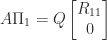
A common method for computing an RRF is QR factorization with column pivoting, which for a matrix A\in\mathbb{R}^{m\times n} with m\ge n computes a factorization A\Pi = QR, where \Pi is a permutation matrix, Q\in\mathbb{R}^{m\times n} has orthonormal columns, and R\in\mathbb{R}^{n\times n} is upper triangular and satisfies the inequalities

\notag    |r_{kk}|^2 \ge \displaystyle\sum_{i=k}^j |r_{ij}|^2,     \quad j=k+1\colon n, \quad k=1\colon n. \qquad (2)

In particular,

\notag   |r_{11}| \ge |r_{22}| \ge \cdots \ge |r_{nn}|.   \qquad(3)

If |r_{kk}| \ge \epsilon \ge |r_{k+1,k+1}| with \epsilon > 0 then we can write

\notag    R =    \begin{array}[b]{@{\mskip33mu}c@{\mskip-16mu}c@{\mskip-10mu}c@{}}    \scriptstyle k &    \scriptstyle n-k &    \\    \multicolumn{2}{c}{        \left[\begin{array}{c@{~}c@{~}}                  R_{11}& R_{12} \\                    0   & R_{22} \\              \end{array}\right]}    & \mskip-12mu\          \begin{array}{c}              \scriptstyle k \\              \scriptstyle n-k              \end{array}    \end{array},  \qquad(4)

with

\notag   \|R_{22}\|_2 \le \|R_{22}\|_F \le 2^{-1/2}(n-k+1)\epsilon.

Hence R is within 2-norm distance 2^{-1/2}(n-k+1)\epsilon of the rank-k matrix \left[\begin{smallmatrix} R_{11} & R_{12} \\ 0 & 0 \end{smallmatrix}\right]. Note that if Q = [Q_1~Q_2] is partitioned conformally with Q in (4) then

\notag   A\Pi =   \begin{bmatrix}    Q_1 & Q_2   \end{bmatrix}   \begin{bmatrix}    R_{11} & R_{12} \\     0     & R_{22} \\   \end{bmatrix}    = Q_1   \begin{bmatrix}    R_{11} & R_{12}   \end{bmatrix}   + \begin{bmatrix}    0 & Q_2 R_{22}   \end{bmatrix},

so \| A\Pi - Q_1 [R_{11}~R_{12}]\|_2 \le \|R_{22}\|_2, which means that Q_1 provides an O(\epsilon) approximation to the range of A.

To assess how good an RRF this factorization is (with p = n) we write it as

\notag   A = QR\Pi^T = Q D Y^T, \quad D = \mathrm{diag}(r_{ii}),                          \quad Y^T = D^{-1}R \Pi^T. \quad (\#)

Applying (1) gives

\notag     \sigma_i(A) = \theta_i \sigma_i(D), \quad i = 1\colon p, \qquad (5)

where \sigma_n(Y)\le \theta_i \le \sigma_1(Y), since Q has orthonormal columns and so has unit singular values. Now D^{-1}R has unit diagonal and, in view of (2), its off-diagonal elements are bounded by 1. Therefore \sigma_1(Y) = \|Y\|_2 \le \|Y\|_F \le (n(n+1)/2)^{1/2}. On the other hand, \sigma_p(Y)^{-1} \le 2^{n-1} by Theorem 1 in Bounds for the Norm of the Inverse of a Triangular Matrix. Therefore

\notag    2^{1-n} \le \theta_i \le (n(n+1)/2)^{1/2}.

The lower bound is an approximate equality for small \tau for the triangular matrix

\notag        R_n(\theta) = \mathrm{diag}(1,s,\dots,s^{n-1})             \begin{bmatrix} 1 & -c & -c     & \dots & -c \\                               & 1  & -c     & \dots & -c \\                               &    & \ddots &\ddots & \vdots \\                               &    &        &\ddots & -c \\                               &    &        &       &  1 \end{bmatrix},      \quad c=\cos\tau, \quad s=\sin\tau,

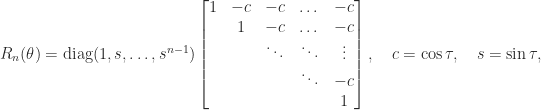
devised by Kahan, which is invariant under QR factorization with column pivoting. Therefore QR factorization with column pivoting is not guaranteed to reveal the rank, and indeed it can fail to do so by an exponentially large factor.

For the matrix (\dagger), QR with column pivoting reorders A to A\Pi = [a_3,~a_4,~a_2,~a_1] and yields

R =
  -3.0000e+00   3.3333e-01   1.3333e+00  -1.6667e+00
            0  -1.6997e+00   2.6149e-01   2.6149e-01
            0            0   1.0742e+00   1.0742e+00
            0            0            0   3.6515e-09

This R suggests a numerical rank of 3 for \epsilon = 10^{-8} (say). In fact, this factorization provides a very good RRF, as in (\#) we have \kappa_2(Y) \approx 3.4.

QR Factorization with Other Pivoting Choices

Consider a QR factorization A\Pi = QR with triangular factor partitioned as

\notag    R =    \begin{array}[b]{@{\mskip33mu}c@{\mskip-16mu}c@{\mskip-10mu}c@{}}    \scriptstyle k &    \scriptstyle n-k &    \\    \multicolumn{2}{c}{        \left[\begin{array}{c@{~}c@{~}}                  R_{11}& R_{12} \\                    0   & R_{22} \\              \end{array}\right]}    & \mskip-12mu\          \begin{array}{c}              \scriptstyle k \\              \scriptstyle n-k              \end{array}    \end{array}. \qquad (6)

We have

\notag    \begin{aligned}      \sigma_{\min}(R_{11}) &\le \sigma_k(A),    \quad \qquad (7)\\      \sigma_{\max}(R_{22}) &\ge \sigma_{k+1}(A), ~\qquad (8)    \end{aligned}

where (7) is from singular value interlacing inequalities and (8) follows from the Eckart-Young theorem, since setting R_{22} to zero gives a rank-k matrix. Suppose A has numerical rank k and \sigma_{k+1} \ll \sigma_k. We would like to be able to detect this situation from R, so clearly we need

\notag  \sigma_{\min}(R_{11}) \approx \sigma_k(A), \quad  \sigma_{\max}(R_{22}) \approx \sigma_{k+1}(A). \qquad (9)

In view of the inequalities (7) and (8) this means that we wish to choose \Pi maximize \sigma_{\min}(R_{11}) and minimize \sigma_{\max}(R_{22}).

Some theoretical results are available on the existence of such QR factorizations. First, we give a result that shows that for k = n-1 the approximations in (9) can hold to within a factor n^{1/2}.

Theorem 1. For A\in\mathbb{R}^{m\times n} with m\ge n there exists a permutation \Pi such that A has the QR factorization A\Pi = QR with |r_{nn}| \le n^{1/2}\sigma_n(A) and \sigma_{\min}(R_{11}) \ge n^{-1/2} \sigma_{n-1}(A), where R_{11} = R(1\colon n-1, 1\colon n-1).

Proof. Let Av = \sigma_n u, with \|v\|_2 = \|u\|_2 = 1 and let \Pi^T be such that \widetilde{v}  = \Pi^Tv satisfies |\widetilde{v}_n| = \|\widetilde{v}\|_{\infty}. Then if A\Pi = QR is a QR factorization,

\notag \begin{aligned}    \sigma_n = \| \sigma_n u \|_2             = \| Av \|_2             = \| QR\Pi^Tv \|_2             = \| R\mskip1mu \widetilde{v} \|_2             \ge | r_{nn} \widetilde{v}_n |             \ge n^{-1/2} | r_{nn} |, \end{aligned}

since \|\widetilde{v}\|_2 = 1, which yields the result.

Next, we write \Pi = [\Pi_1~\pi], where \pi\in\mathbb{R}^n, and partition

\notag   R = \begin{bmatrix}    R_{11} & R_{12} \\     0     & R_{22} \\   \end{bmatrix}

with R_{11}\in\mathbb{R}^{(n-1)\times (n-1)}. Then

A\Pi_1 = Q \begin{bmatrix} R_{11} \\ 0 \end{bmatrix}

implies \sigma_{\min}(A\Pi_1) = \sigma_{\min}(R_{11}). On the other hand, if A = U\Sigma V^T is an SVD with U\in\mathbb{R}^{m\times n}, \Sigma = \mathrm{diag}(D_1,\sigma_n)\in\mathbb{R}^{n\times n}, and V = [V_1~v] then

\notag  A\Pi_1 = U\Sigma V^T \Pi_1 =    U    \begin{bmatrix}    D_1    & 0 \\     0     & \sigma_n \\   \end{bmatrix}   \begin{bmatrix}    V_1^T \\ v^T   \end{bmatrix} \Pi_1   = U   \begin{bmatrix}    D_1V_1^T \\ \sigma_n v^T   \end{bmatrix} \Pi_1,

so

\notag   \sigma_{\min}(A\Pi_1) =   \sigma_{\min}\left(   \begin{bmatrix}    D_1V_1^T \\ \sigma_n v^T   \end{bmatrix} \Pi_1 \right)    \ge \sigma_{\min}(D_1V^T\Pi_1)    \ge \sigma_{n-1}\sigma_{\min}(V^T\Pi_1).

Finally, we note that we can partition the orthogonal matrix V^T\Pi_1 as

\notag  V^T\Pi =    \begin{bmatrix}    V_1^T\Pi_1  & V_1^T\pi \\    v^T\Pi_1    & v^T\pi   \end{bmatrix},

and the CS decomposition implies that

\notag    \sigma_{\min}(V_1^T\Pi_1) =    \sigma_{\min}(v^T\pi) =    |v^T\pi| = |\widetilde{v}_n| \ge n^{-1/2}.

Hence \sigma_{\min}(R_{11}) \ge n^{-1/2} \sigma_{n-1}, as required. ~\square

Theorem 1 is a special case of the next result of Hong and Pan (1992).

Theorem 2. For A\in\mathbb{R}^{m\times n} with m\ge n and any k there exists a permutation matrix \Pi such that A has the QR factorization A\Pi = QR where, with R partitioned as in (6),

\notag    \sigma_{\max}(R_{22}) \le f(k,n) \sigma_{k+1}(A), \quad    \sigma_{\min}(R_{11}) \ge f(k,n)^{-1} \sigma_k(A),

where f(k,n) = (k(n-k) + \min(k,n-k))^{1/2}.

The proof of Theorem 2 is constructive and chooses \Pi to move a submatrix of maximal determinant of V_2 to the bottom of V_2, where V_2 comprises the last n-k columns of the matrix of right singular vectors.

Theorem 2 shows the existence of an RRF up to the factor f(k,n) \le (n+1)/2, but it does not provide an efficient algorithm for computing one.

Much work has been done on algorithms that choose the permutation matrix \Pi in a different way to column pivoting or post-process a QR factorization with column pivoting, with the aim of satisfying (9) at reasonable cost. Typically, these algorithms involve estimating singular values and singular vectors. We are not aware of any algorithm that is guaranteed to satisfy (9) and requires only O(n^3) flops.

UTV Decomposition

By applying Householder transformations on the right, a QR factorization with column pivoting can be turned into a complete orthogonal decomposition of
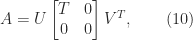
 A\in\mathbb{R}^{m\times n}, which has the form

\notag      A = U \begin{bmatrix} T & 0 \\ 0 & 0 \end{bmatrix} V^T, \qquad (10)

where T\in\mathbb{R}^{r \times r} is upper triangular and U\in\mathbb{R}^{m\times m} and V\in\mathbb{R}^{n\times n} are orthogonal. Stewart (1998) calls (6) with T upper triangular or lower triangular a UTV decomposition and he defines a rank-revealing UTV decomposition of numerical rank r by

\notag \begin{aligned}      A &= U \begin{bmatrix} T & F \\ 0 & G  \end{bmatrix} V^T,          \qquad T\in\mathbb{R}^{r \times r}, \\         &          \sigma_r(T) \approx \sigma_r(A), \quad          \|F\|_F^2 + \|G\|_F^2 \approx \sigma_{r+1}^2 + \cdots + \sigma_n^2. \end{aligned}

The UTV decomposition is easy to update (when a row is added) and downdate (when a row is removed) using Givens rotations and it is suitable for parallel implementation. Initial determination of the UTV decomposition can be done by applying the updating algorithm as the rows are brought in one at a time.

LU Factorization

Instead of QR factorization we can build an RRF from an LU factorization with pivoting. For A\in\mathbb{R}^{m\times n} with m\ge n, let

\notag     \Pi_1 A \Pi_2 = LU =     \begin{bmatrix}       L_{11} & 0 \\       L_{12} & L_{22}     \end{bmatrix}     \begin{bmatrix}     U_{11} & U_{12}\\       0    & U_{22}     \end{bmatrix},

where \Pi_1 and \Pi_2 are permutation matrices, L and U are m\times n lower and n\times n upper triangular, respectively, and L_{11} and U_{11} are k\times k. Analogously to (7) and (8), we always have \sigma_{\min}(L_{11}U_{11}) \le \sigma_k(A) and \sigma_{\max}(L_{22}U_{22}) \ge \sigma_{k+1}(A). With a suitable pivoting strategy we can hope that \sigma_{\min}(L_{11}U_{11}) \approx \sigma_k(A) and \sigma_{\max}(L_{22}U_{22}) \approx \sigma_{k+1}(A).

A result of Pan (2000) shows that an RRF based on LU factorization always exists up to a modest factor f(k,n). This is analogue for LU factorization of Theorem 2.

Theorem 3 For A\in\mathbb{R}^{m\times n} with m\ge n and any k there exist permutation matrices \Pi_1 and \Pi_2 such that

\notag     \Pi_1 A \Pi_2 = LU =     \begin{bmatrix}     L_{11} &  0    \\     L_{12} & I_{m-k,n-k}     \end{bmatrix}    \begin{array}[b]{@{\mskip33mu}c@{\mskip-16mu}c@{\mskip-10mu}c@{}}    \scriptstyle k &    \scriptstyle n-k &    \\    \multicolumn{2}{c}{        \left[\begin{array}{c@{~}c@{~}}                  U_{11}& U_{12} \\                    0   & U_{22} \\              \end{array}\right]}    & \mskip-12mu\          \begin{array}{c}              \scriptstyle k \\              \scriptstyle n-k              \end{array}    \end{array},

where L_{11} is unit lower triangular, U_{11} is upper triangular, and

\notag    \sigma_{\max}(U_{22}) \le f(k,n) \sigma_{k+1}(A), \quad    \sigma_{\min}(L_{11}U_{11}) \ge f(k,n)^{-1} \sigma_k(A),

where f(k,n) = k(n-k) + 1.

Again the proof is constructive, but the permutations it chooses are too expensive to compute. In practice, complete pivoting often yields a good RRF.

In terms of Definition 1, an RRF has

\notag     X = \Pi_1^TL D, \quad D = \mathrm{diag}(u_{ii}), \quad     Y^T = D^{-1}U\Pi_2. \qquad (\ddagger)

For the matrix (\dagger), the U factor for LU factorization without pivoting is

U =
   1.0000e+00   1.0000e+00   1.0000e-08            0
            0  -2.0000e+00   2.0000e+00   1.0000e+00
            0            0   5.0000e-09  -1.5000e+00
            0            0            0  -2.0000e+00

As for QR factorization without pivoting, an RRF is not obtained from (\ddagger).. However, with complete pivoting we obtain

U =
   2.0000e+00   1.0000e+00  -1.0000e+00   1.0000e+00
            0  -2.0000e+00            0            0
            0            0   1.0000e+00   1.0000e+00
            0            0            0  -5.0000e-09

which yields a very good RRF (\ddagger) with \kappa_2(X) = 3.5 and \kappa_2(Y) = 3.4.

Notes

QR factorization with column pivoting is difficult to implement efficiently, as the criterion for choosing the pivots requires the norms of the active parts of the remaining columns and this requires a significant amount of data movement. In recent years, randomized RRF algorithms have been developed that use projections with random matrices to make pivot decisions based on small sample matrices and thereby reduce the amount of data movement. See, for example, Martinsson et al. (2019).

References

This is a minimal set of references, which contain further useful references within.

Related Blog Posts

This article is part of the “What Is” series, available from https://nhigham.com/category/what-is and in PDF form from the GitHub repository https://github.com/higham/what-is.

My Blog Workflow

This blog, which I started in 2013, is hosted on wordpress.com. WordPress sites are both websites and blogs, and in late 2020 I translated my website over to this same domain name (nhigham.com).

org2blog_logo-color-multi.png

The whole site is maintained as Emacs Org mode files that I export to WordPress using the Emacs org2blog package. I do not use the WordPress editor, except occasionally to copy the html for a figure back into an Org file for tweaking and re-exporting as html (usually in order to have text next to an image, as here).

WordPress supports \LaTeX math mode, which must be typed within single dollar signs with the word “latex” right after the first dollar sign. Emacs Org mode supports \LaTeX equations and Org2blog does an excellent job of exporting to WordPress with the necessary conversions. For example, to produce the displayed equation

\notag  X =  \begin{bmatrix}        a_{11} & a_{12} \\        a_{12} & a_{22}       \end{bmatrix}^{-1}

I type

\begin{equation}\notag
 X =  \begin{bmatrix}
       a_{11} & a_{12} \\ 
       a_{12} & a_{22} 
      \end{bmatrix}^{-1}
\end{equation}

in my source and this is converted into

wordpress_eqn_example.jpg

in WordPress. (This fragment is included as an image because if I include the text directly I cannot stop WordPress interpreting it as \LaTeX!)

The beauty of this workflow is that I can export this same source to html, \LaTeX (then PDF), or even a Word file using Org mode’s export dispatcher. This is how I produce the PDF versions of the posts in the What Is series.

Advantages of this workflow are

  • I can work almost entirely in Emacs and avoid using the WordPress editor.
  • Org mode files are very readable and easy to edit.
  • Org2blog automatically uploads images into the WordPress media library and links to them.
  • Raw html can be included.

Drawbacks of the workflow are

  • \LaTeX macros cannot be defined, so \LaTeX commands must always be typed in full.
  • Displayed equations must be typed in an equation environment for reliable results.
  • All math is formatted in text style, so \displaystyle must be put in front of every \frac, \sum, etc. to obtain display style (so that formulas in fractions are not set in a smaller font, for example).
  • Inline math has awkward vertical spacing.
  • In the current version of org2blog, equation* (for an unnumbered equation) is not supported.

The latter three disadvantages would be avoided if the \LaTeX was interpreted by MathJax, but this requires a MathJax plugin, and the Business Plan is needed to be able to install plugins (I have the Premium plan).

Here is what the Emacs Org mode source code looks like for the post What Is the Sylvester Equation? After the properties drawer, which contains information about the post on WordPress, the text looks like standard \LaTeX, with the exception that a comment line begins with the # symbol rather than %.

what-is-kron_src.jpg

Singular Value Inequalities

Recall that the singular value decomposition (SVD) of a matrix A \in\mathbb{C}^{m\times n} is a factorization A = U\Sigma V^*, where U\in\mathbb{C}^{m\times m} and V\in\mathbb{C}^{n\times n} are unitary and \Sigma = \mathrm{diag}(\sigma_1,\dots, \sigma_p)\in\mathbb{R}^{m\times n}, with \sigma_1\ge \sigma_2\ge \cdots \ge \sigma_p \ge 0, where where p = \min(m,n). We sometimes write \sigma_i(A) to specify the matrix to which the singular value belongs.

A standard technique for obtaining singular value inequalities for A is to apply eigenvalue inequalities to the Hermitian positive semidefinite matrices A^*A or AA^*, whose eigenvalues are the squares of the singular values of
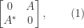
 A, or to the Hermitian matrix

\notag    \begin{bmatrix}      0   & A \\      A^* & 0     \end{bmatrix}, \qquad (1)

whose eigenvalues are plus and minus the singular values of A together with |m-n| zero eigenvalues if m\ne n.

We begin with a variational characterization of singular values.

Theorem 1. For A\in\mathbb{C}^{m\times n},

\notag \begin{aligned}   \sigma_k &= \min_{\dim(S)=n-k+1} \, \max_{0\ne x\in S} \frac{\|Ax\|_2}{\|x\|_2}\\            &= \max_{\dim(S)= k} \, \min_{0\ne x\in S} \frac{\|Ax\|_2}{\|x\|_2},                  \quad k=1\colon \min(m,n), \end{aligned}

where S\subseteq \mathbb{C}^n.

Proof. The result is obtained by applying the Courant–Fischer theorem (a variational characterization of eigenvalues) to A^*A. ~\square

As a special case of Theorem 1, we have

\notag    \sigma_1 = \displaystyle\max_{x \ne 0}\frac{ \|Ax\|_2 }{ \|x\|_2 },               \qquad (2)

and, for m\ge n,

\notag    \sigma_n = \displaystyle\min_{x \ne 0}\frac{ \|Ax\|_2 }{ \|x\|_2 }.               \qquad (3)

The expression in the theorem can be rewritten using \|x\|_2 = \max_{y\ne 0}|y^*x|/\|y\|_2 (the equality case in the Cauchy–Schwarz inequality). For example, (2) is equivalent to
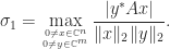
\notag   \sigma_1 = \displaystyle\max_{0\ne x\in \mathbb{C}^n\atop 0 \ne y \in \mathbb{C}^m}         \displaystyle\frac{|y^*Ax|}{\|x\|_2\|y\|_2}.

Our first perturbation result bounds the change in a singular value.

Theorem 2. For A,B\in\mathbb{C}^{m\times n},

\notag   |\sigma_i(A) - \sigma_i(B)| \le \|A - B \|_2, \quad i = 1\colon \min(m,n).    \qquad (4)

Proof. The bound is obtained by applying the corresponding result for the Hermitian eigenvalue problem to (1). ~\square

The bound (4) says that the singular values of a matrix are well conditioned under additive perturbation. Now we consider multiplicative perturbations.

The next result is an analogue for singular values of Ostrowski’s theorem for eigenvalues.

Theorem 3. For A\in \mathbb{C}^{m\times n} and nonsingular X\in\mathbb{C}^{n\times n} and Y\in\mathbb{C}^{m\times m},

\notag     \sigma_i(Y^*AX) = \theta_i \sigma_i(A), \quad i = 1\colon \min(m,n),      \qquad (5)

where \sigma_n(X)\sigma_m(Y) \le \theta_i \le \sigma_1(X) \sigma_1(Y).

A corollary of this result is

\notag   |\sigma_i(A) - \sigma_i(Y^*AX)| \le \sigma_i(A) \epsilon, \quad i = 1\colon \min(m,n),    \qquad (6)

where \epsilon = \max(\|X^*X - I\|_2,\|Y^*Y - I\|_2). The bounds (5) and (6) are intuitively reasonable, because unitary transformations preserve singular values and the bounds quantify in different ways how close X and Y are to being unitary.

Next, we have an interlacing property.

Theorem 4. Let A\in\mathbb{C}^{m\times n}, A_k = A(:,1\colon k), and q = \min(m,k). Then

\notag  \sigma_{i+1}(A_{k+1}) \le \sigma_i(A_k) \le \sigma_i(A_{k+1}), \quad   i=1\colon q, \quad k = 1\colon n-1,

where we define \sigma_{q+1}(A_{k+1}) = 0 if m < k+1.

Proof. The result is obtained by applying the Cauchy interlace theorem to A^*A, noting that A_k^*A_k is the leading principal submatrix of order k of A^*A. ~\square

An analogous result holds with rows playing the role of columns (just apply Theorem 4 to A^*).

Theorem 4 encompasses two different cases, which we illustrate with i = q and k = n-1. The first case is m \ge n, so that q = n-1 and

\notag   \sigma_n(A) \le \sigma_{n-1}(A_{n-1}) \le \sigma_{n-1}(A).

The second case is m < n, so q = m and

\notag   0 \le \sigma_m(A_{n-1}) \le \sigma_m(A).

Therefore Theorem 3 shows that removing a column from A does not increase any singular value and that when m\ge n no singular value decreases below \sigma_n(A). However, when m < n the smallest singular value of A_{n-1} may be less than the smallest singular value of A.

Here is a numerical example. Note that transposing A does not change its singular values.

>> rng(1), A = rand(5,4); % Case 1.
>> B = A(:,1:end-1); sv_A = svd(A)', sv_B = svd(B)'
sv_A =
   1.7450e+00   6.4492e-01   5.5015e-01   3.2587e-01
sv_B =
   1.5500e+00   5.8472e-01   3.6128e-01
> A = A'; B = A(:,1:end-1); sv_B = svd(B)' % Case 2
sv_B =
   1.7098e+00   6.0996e-01   4.6017e-01   1.0369e-01

By applying Theorem 4 repeatedly we find that if we partition A = [A_{11}~A_{12}] then \sigma_i(A_{11}) \le \sigma_i(A) for all i for which the left-hand side is defined.

References