Gaussian elimination is the process of reducing an 


James Wilkinson showed in the early 1960s that the numerical stability of Gaussian elimination depends on the growth factor
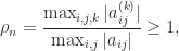
where the 


If no row interchanges are done during the elimination then 

- If
is symmetric positive definite then
. In this case one would normally use Cholesky factorization instead of LU factorization.
- If
- If
.
- If
.
The entry in the 
Partial Pivoting
Partial pivoting interchanges rows to ensure that the pivot element is the largest in magnitude in its column. Wilkinson showed that partial pivoting ensures 

![\left[\begin{array}{@{\mskip3mu}rrrr} 1 & 0 & 0 & 1 \\ -1 & 1 & 0 & 1 \\ -1 & -1 & 1 & 1 \\ -1 & -1 & -1 & 1 \\ \end{array} \right].](https://s0.wp.com/latex.php?latex=%5Cleft%5B%5Cbegin%7Barray%7D%7B%40%7B%5Cmskip3mu%7Drrrr%7D+++++++++++++++++++++++1++%26+0++%26+0++%26+1++%5C%5C+++++++++++++++++++++++-1+%26+1++%26+0++%26+1++%5C%5C+++++++++++++++++++++++-1+%26+-1+%26+1++%26+1++%5C%5C+++++++++++++++++++++++-1+%26+-1+%26+-1+%26+1++%5C%5C++++++++%5Cend%7Barray%7D++++++++%5Cright%5D.+&bg=ffffff&fg=222222&s=0&c=20201002)
This matrix is a special case of a larger class of matrices for which equality is attained (Higham and Higham, 1989). Exponential growth can occur for matrices arising in practical applications, as shown by Wright for the multiple shooting method for two-point boundary value problems and Foster for a quadrature method for solving Volterra integral equations. Remarkably, though,
Rook Pivoting
Rook pivoting interchanges rows and columns to ensure that the pivot element is the largest in magnitude in both its row and its column. Foster has shown that

This bound grows much more slowly than the bound for partial pivoting, but it can still be large. In practice, the bound is pessimistic.
Complete Pivoting
Complete pivoting chooses as pivot the largest element in magnitude in the remaining part of the matrix. Wilkinson (1961) showed that

This bound grows much more slowly than that for rook pivoting, but again it is pessimistic. Wilkinson noted in 1965 that no matrix had been discovered for which 


That 

Growth Factor Bounds for Any Pivoting Strategy
While much attention has focused on investigating the growth factor for particular pivoting strategies, some results are known that provide growth factor lower bounds for any pivoting strategy. Higham and Higham (1989) obtained a result that implies that for the symmetric orthogonal matrix
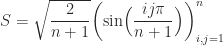
the lower bound
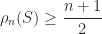
holds for any pivoting strategy. Recently, Higham, Higham, and Pranesh (2020) have shown that
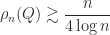
with high probability for large 

gallery('randsvd',n,kappa,2) in MATLAB.
Experimentation
If you want to experiment with growth factors in MATLAB, you can use the function gep from the Matrix Computation Toolbox. Examples:
>> rng(0); A = randn(1000);
>> [L,U,P,Q,rho] = gep(A,'p'); rho  % Partial pivoting.
rho =
   1.9437e+01
>> [L,U,P,Q,rho] = gep(A,'r'); rho  % Rook pivoting.
rho =
   9.9493e+00
>> [L,U,P,Q,rho] = gep(A,'c'); rho  % Complete pivoting.
rho =
   6.8363e+00
>> A = gallery('randsvd',1000,1e1,2);
>> [L,U,P,Q,rho] = gep(A,'c'); rho  % Complete pivoting.
rho =
   5.4720e+01
References
This is a minimal set of references, which contain further useful references within.
- Alan Edelman, The complete pivoting conjecture for Gaussian elimination is false, The Mathematica Journal 2, 58–61, 1992.
- Leslie V. Foster, The growth factor and efficiency of Gaussian elimination with rook pivoting, J. Comput. Appl. Math. 86, 177–194, 1997
- Nicholas J. Higham and Desmond J. Higham, Large growth factors in Gaussian elimination with pivoting, SIAM J. Matrix Anal. Appl. 10 (2), 155–164, 1989.
- Desmond J. Higham, Nicholas J. Higham, and Srikara Pranesh, Random Matrices Generating Large Growth in LU Factorization with Pivoting, MIMS EPrint 2020.13, The University of Manchester, UK, May 2020.
- Nicholas J. Higham, Accuracy and Stability of Numerical Algorithms, second edition, Society for Industrial and Applied Mathematics, Philadelphia, PA, USA, 2002. Sections 9.4, 10.4.
- Christos Kravvaritis and Marilena Mitrouli, The growth factor of a Hadamard matrix of order
is
- J. H. Wilkinson, Error analysis of direct methods of matrix inversion, J. Assoc. Comput. Mach. 8, 281–330, 1961.
Related Blog Posts
- Randsvd Matrices with Large Growth Factors (2020)
- What Is a Hadamard Matrix? (2020)
- What Is a Random Orthogonal Matrix? (2020)
This article is part of the “What Is” series, available from https://nhigham.com/category/what-is and in PDF form from the GitHub repository https://github.com/higham/what-is.

Hi Sirs.
There must be some bug in the “gep” function when rook pivoting is chosen.
In the example
rng(0); A = randn(1000);
[L,U,P,Q,rho] = gep(A,’r’); rho % Rook pivoting.
a warning “too many FOR loop iterations” is issued.
There was a change in MATLAB a while back to the allowed limits in for loops. I hope to do a major update of the toolbox later this year. For now you can get an updated gep.m from https://www.dropbox.com/s/pqwilyyjg66v9y1/gep.m?dl=0
Thanks Nick. That would be great. I’ll use this version in the meantime.